SQL Window Functions: RANK vs DENSE_RANK, LAG/LEAD, and Frame Clauses

A window function computes a value across a set of rows related to the current row, and returns that value on every row instead of collapsing them. That single property — rows survive — is what GROUP BY cannot do, and it is why window functions show up so constantly in data interviews at Meta, Amazon, DoorDash, and TikTok. This guide works through the ones interviewers actually ask: the ranking trio and how each handles ties, LAG/LEAD for row-to-row comparisons, and the frame clause that quietly changes your running total.

Every query below runs as written against the inline sample tables. Result sets are the real output from PostgreSQL 16.

Key Takeaways

• ROW_NUMBER, RANK, and DENSE_RANK produce identical output until two rows tie. Interviewers create the tie on purpose, so pick by what "top N" means: N rows is ROW_NUMBER, N distinct values is DENSE_RANK.
• ROW_NUMBER is non-deterministic when the window's ORDER BY has ties. Add a unique tiebreaker column or your "latest record per user" query returns a different row on a different day.
• The default frame with ORDER BY is RANGE BETWEEN UNBOUNDED PRECEDING AND CURRENT ROW, not ROWS. With duplicate sort keys, a running total counts rows that have not been printed yet.
• ROWS BETWEEN 6 PRECEDING AND CURRENT ROW counts rows, not days. If a date is missing from the table, your "7-day moving average" silently averages 7 rows spanning 9 days.
• Window functions run after WHERE, GROUP BY, and HAVING, so none of those clauses can see them. Wrap the query in a CTE or subquery and filter there.

A window function computes across rows without destroying them

Asked at Amazon — Compute join counts and window ranks A short schema of customers, orders, and a scores table is given, and you have to state exact row counts for several joins and then produce window-ranked output over the scores. The interviewer is checking two things at once: that you can predict join cardinality, and that you understand a window function does not change the number of rows going out.

Start with the contrast, because it is the mental model everything else hangs on.

CREATE TABLE employees (name TEXT, dept TEXT, salary INT);
INSERT INTO employees VALUES
  ('Ada','Data',175000), ('Bo','Data',160000), ('Chen','Data',160000), ('Dara','Data',145000),
  ('Eli','Infra',190000), ('Fay','Infra',165000), ('Gus','Infra',165000);

GROUP BY gives you one row per department and throws the employees away:

SELECT dept, AVG(salary)::int AS dept_avg
FROM employees
GROUP BY dept
ORDER BY dept;

 dept  | dept_avg
-------+----------
 Data  |   160000
 Infra |   173333
(2 rows)

The same aggregate in an OVER() clause keeps all seven employees and attaches the department average to each one:

SELECT name, dept, salary,
       AVG(salary) OVER (PARTITION BY dept)::int AS dept_avg
FROM employees
ORDER BY dept, salary DESC, name;

 name | dept  | salary | dept_avg
------+-------+--------+----------
 Ada  | Data  | 175000 |   160000
 Bo   | Data  | 160000 |   160000
 Chen | Data  | 160000 |   160000
 Dara | Data  | 145000 |   160000
 Eli  | Infra | 190000 |   173333
 Fay  | Infra | 165000 |   173333
 Gus  | Infra | 165000 |   173333
(7 rows)

Seven rows in, seven rows out. That is the whole idea. Any question phrased as "show each row and its share of / rank within / difference from the group" is a window function question, because the alternative is a self-join back to an aggregated subquery.

Video companion: This verified YouTube video gives a second pass on the same prep area.

The anatomy of OVER()

OVER() has three parts, and each one is optional:

<function>() OVER (
  PARTITION BY <cols>   -- split rows into independent groups
  ORDER BY    <cols>    -- order rows inside each group
  ROWS|RANGE  <frame>   -- restrict which ordered rows are visible
)

• PARTITION BY splits the table into groups that never see each other. Omit it and the whole result set is one partition.
• ORDER BY sequences rows inside the partition. Plain aggregates do not need it. Ranking and navigation functions are meaningless without it, though PostgreSQL will not stop you: ROW_NUMBER() OVER () runs happily and numbers the rows in whatever order they arrive. SQL Server rejects that outright. Treat it as required even where the engine does not.
• The frame narrows the visible rows further. Omit it and you get one of two defaults, which is the trap covered further down.

If you use the same window twice, name it once with a WINDOW clause:

SELECT name, dept, salary,
       SUM(salary) OVER w AS dept_total,
       ROUND(100.0 * salary / SUM(salary) OVER w, 1) AS pct_of_dept,
       COUNT(*) OVER () AS total_rows
FROM employees
WINDOW w AS (PARTITION BY dept)
ORDER BY dept, salary DESC, name;

 name | dept  | salary | dept_total | pct_of_dept | total_rows
------+-------+--------+------------+-------------+------------
 Ada  | Data  | 175000 |     640000 |        27.3 |          7
 Bo   | Data  | 160000 |     640000 |        25.0 |          7
 Chen | Data  | 160000 |     640000 |        25.0 |          7
 Dara | Data  | 145000 |     640000 |        22.7 |          7
 Eli  | Infra | 190000 |     520000 |        36.5 |          7
 Fay  | Infra | 165000 |     520000 |        31.7 |          7
 Gus  | Infra | 165000 |     520000 |        31.7 |          7
(7 rows)

Naming the window is a readability win, not a performance one — PostgreSQL collapses identical window specifications whether you wrote them inline or named them, and both forms above plan to the same single Sort feeding a single WindowAgg. What costs you is a spec that differs. Change one function's ORDER BY and EXPLAIN grows a second Sort stacked on a second WindowAgg; on a wide fact table that is one pass turning into two. The WINDOW clause helps because it makes an accidental divergence impossible to introduce by editing one copy of three.

ROW_NUMBER, RANK, and DENSE_RANK differ only when values tie

Asked at Meta — Resolve Ties for Top-10 Users in SQL Query An Oculus scores table holds one score per user, and you have to return exactly ten users for a leaderboard when the users at ranks 10 and 11 have the same score. The interviewer wants you to say out loud which ranking function you chose and what happens to the tied user you excluded. There is no single correct answer, only a correct justification.

Ties are the entire exam. Put all three functions in one result set and the difference is obvious:

SELECT name, dept, salary,
       ROW_NUMBER() OVER (PARTITION BY dept ORDER BY salary DESC) AS rn,
       RANK()       OVER (PARTITION BY dept ORDER BY salary DESC) AS rnk,
       DENSE_RANK() OVER (PARTITION BY dept ORDER BY salary DESC) AS dns
FROM employees
ORDER BY dept, salary DESC, name;

 name | dept  | salary | rn | rnk | dns
------+-------+--------+----+-----+-----
 Ada  | Data  | 175000 |  1 |   1 |   1
 Bo   | Data  | 160000 |  2 |   2 |   2
 Chen | Data  | 160000 |  3 |   2 |   2
 Dara | Data  | 145000 |  4 |   4 |   3
 Eli  | Infra | 190000 |  1 |   1 |   1
 Fay  | Infra | 165000 |  2 |   2 |   2
 Gus  | Infra | 165000 |  3 |   2 |   2
(7 rows)

Look at Dara. RANK gives 4 because two people occupied position 2 and position 3 was consumed. DENSE_RANK gives 3 because 145000 is the third-highest salary. ROW_NUMBER gives 4 because it is counting rows and does not care about the values at all.

The mistake: assuming ROW_NUMBER is deterministic

ROW_NUMBER assigned Bo 2 and Chen 3 above. Nothing in the SQL standard guarantees that. The window's ORDER BY salary DESC cannot separate two rows at 160000, so the engine picks an order, and it may pick differently after a vacuum, a plan change, or a parallel scan.

This matters most in the pattern people use ROW_NUMBER for the most — keeping the latest row per key. If two rows share the maximum timestamp, "the latest record" is a coin flip. Break the tie explicitly:

SELECT name, dept, salary,
       ROW_NUMBER() OVER (PARTITION BY dept ORDER BY salary DESC, name) AS rn
FROM employees
ORDER BY dept, salary DESC, name;

 name | dept  | salary | rn
------+-------+--------+----
 Ada  | Data  | 175000 |  1
 Bo   | Data  | 160000 |  2
 Chen | Data  | 160000 |  3
 Dara | Data  | 145000 |  4
 Eli  | Infra | 190000 |  1
 Fay  | Infra | 165000 |  2
 Gus  | Infra | 165000 |  3
(7 rows)

Same numbers, but now they are reproducible. Saying this unprompted is a strong signal; most candidates never mention it.

Two ranking patterns interviewers ask by name

Ranking is rarely the deliverable. It is the middle step of one of two shapes: keep the best few per group, or keep exactly one row per key. Both are built from the functions above, and each has a characteristic wrong answer.

Top-N per group: "top 3" rarely means three rows

Asked at Amazon — Find Top-3 Salaries Per Department Using SQL Given an employees table with a department column, return the top three salary amounts in each department, and the prompt explicitly allows more than three people to come back when they tie on an amount. That parenthetical is the question. It tells you the unit being counted is the salary value, not the employee.

Read the phrasing before you write anything. "Top 3 salaries" and "top 3 employees" are different queries, and the difference shows up only on tied data.

DENSE_RANK counts distinct amounts, which is what this prompt asked for:

WITH ranked AS (
  SELECT name, dept, salary,
         DENSE_RANK() OVER (PARTITION BY dept ORDER BY salary DESC) AS salary_rank
  FROM employees
)
SELECT name, dept, salary, salary_rank
FROM ranked
WHERE salary_rank <= 3
ORDER BY dept, salary_rank, name;

 name | dept  | salary | salary_rank
------+-------+--------+-------------
 Ada  | Data  | 175000 |           1
 Bo   | Data  | 160000 |           2
 Chen | Data  | 160000 |           2
 Dara | Data  | 145000 |           3
 Eli  | Infra | 190000 |           1
 Fay  | Infra | 165000 |           2
 Gus  | Infra | 165000 |           2
(7 rows)

Swap in RANK() and change nothing else. Dara disappears:

WITH ranked AS (
  SELECT name, dept, salary,
         RANK() OVER (PARTITION BY dept ORDER BY salary DESC) AS salary_rank
  FROM employees
)
SELECT name, dept, salary, salary_rank
FROM ranked
WHERE salary_rank <= 3
ORDER BY dept, salary_rank, name;

 name | dept  | salary | salary_rank
------+-------+--------+-------------
 Ada  | Data  | 175000 |           1
 Bo   | Data  | 160000 |           2
 Chen | Data  | 160000 |           2
 Eli  | Infra | 190000 |           1
 Fay  | Infra | 165000 |           2
 Gus  | Infra | 165000 |           2
(6 rows)

145000 is unambiguously the third-highest salary in Data, and RANK dropped it because the tie at 160000 consumed rank 3. This is the single most common wrong answer to top-N-per-group, and it only ever surfaces on tied data, which is exactly why interviewers seed the sample table with a tie.

Dedup to the latest row per key: ROW_NUMBER's real job

Asked at Meta — Write SQL to analyze shop visibility A shop visibility log records a 0/1 state per profile with a timestamp, and you have to determine each shop's current state as of a cutoff while ignoring consecutive rows that repeat the same value. Two separate window patterns fall out of it: ROW_NUMBER for the current state, and LAG for detecting genuine flips.

Change-log tables have many rows per entity and you usually want one. ROW_NUMBER ordered descending, filtered to 1, is the standard answer.

CREATE TABLE shop_visibility (profile_id INT, ts TIMESTAMP, visibility INT);
INSERT INTO shop_visibility VALUES
  (1,'2026-03-01 09:00',1), (1,'2026-03-04 11:00',0),
  (1,'2026-03-04 15:00',0), (1,'2026-03-09 08:00',1),
  (2,'2026-03-02 10:00',1), (2,'2026-03-05 12:00',0);

WITH ranked AS (
  SELECT profile_id, ts, visibility,
         ROW_NUMBER() OVER (PARTITION BY profile_id ORDER BY ts DESC) AS rn
  FROM shop_visibility
)
SELECT profile_id, ts, visibility
FROM ranked
WHERE rn = 1
ORDER BY profile_id;

 profile_id |         ts          | visibility
------------+---------------------+------------
          1 | 2026-03-09 08:00:00 |          1
          2 | 2026-03-05 12:00:00 |          0
(2 rows)

Here ROW_NUMBER is correct and DENSE_RANK is wrong, which is the reverse of the top-N case: if a profile had two rows at the same timestamp, DENSE_RANK would return both and quietly duplicate the entity. ROW_NUMBER returns exactly one, which is what "one row per profile" means. Add the tiebreaker anyway so you know which one.

Postgres also has DISTINCT ON (profile_id) ... ORDER BY profile_id, ts DESC, which is shorter and often faster. It is Postgres-only, so use it when the interviewer says Postgres and reach for ROW_NUMBER when they say ANSI SQL.

LAG and LEAD replace the self-join for row-to-row comparisons

Asked at DoorDash — Write SQL for percent and window changes An exposures table and an orders table are given, and the prompt requires CTEs plus several window functions to produce percent changes across days for treatment and control units. The percent-change column is where candidates lose points, usually by dividing without guarding the denominator.

LAG(col) reads the previous row in the window; LEAD(col) reads the next. Both take an optional offset and an optional default for when there is no such row.

CREATE TABLE daily_orders (dt DATE, orders INT);
INSERT INTO daily_orders VALUES
  ('2026-03-01',120), ('2026-03-02',150), ('2026-03-03',138),
  ('2026-03-06',200), ('2026-03-07',210);

SELECT dt, orders,
       LAG(orders) OVER (ORDER BY dt) AS prev_orders,
       orders - LAG(orders) OVER (ORDER BY dt) AS delta,
       ROUND(100.0 * (orders - LAG(orders) OVER (ORDER BY dt))
             / NULLIF(LAG(orders) OVER (ORDER BY dt), 0), 1) AS pct_change
FROM daily_orders
ORDER BY dt;

     dt     | orders | prev_orders | delta | pct_change
------------+--------+-------------+-------+------------
 2026-03-01 |    120 |        NULL |  NULL |       NULL
 2026-03-02 |    150 |         120 |    30 |       25.0
 2026-03-03 |    138 |         150 |   -12 |       -8.0
 2026-03-06 |    200 |         138 |    62 |       44.9
 2026-03-07 |    210 |         200 |    10 |        5.0
(5 rows)

Three things to say out loud when you write this:

The first row is NULL and that is correct. There is no previous day. If the spec wants 0 instead, use the third argument: LAG(orders, 1, 0).

NULLIF on the denominator is not optional. A day with zero orders makes the denominator zero, and Postgres aborts the whole query with division by zero rather than returning NULL — that holds for numeric division as much as integer division, so the decimal literal in front does not save you.

Row order is not date order. Look at 2026-03-06: its "previous" row is 2026-03-03, three days earlier, because 03-04 and 03-05 have no rows at all. LAG walks rows, not calendar days.

That last point is a bug in most candidates' day-over-day queries, and it is also the tool for the opposite task. Subtract the lagged date and gaps announce themselves:

SELECT dt,
       LAG(dt) OVER (ORDER BY dt) AS prev_dt,
       dt - LAG(dt) OVER (ORDER BY dt) AS day_gap
FROM daily_orders
ORDER BY dt;

     dt     |  prev_dt   | day_gap
------------+------------+---------
 2026-03-01 | NULL       |    NULL
 2026-03-02 | 2026-03-01 |       1
 2026-03-03 | 2026-03-02 |       1
 2026-03-06 | 2026-03-03 |       3
 2026-03-07 | 2026-03-06 |       1
(5 rows)

Any day_gap > 1 is an inactivity window, which is how churn definitions like "no activity for N days" get implemented without a calendar table. The same shape solves the Meta shop-visibility requirement to ignore repeated states — compare each row to its predecessor and keep only the rows where the value actually changed:

WITH flagged AS (
  SELECT profile_id, ts, visibility,
         LAG(visibility) OVER (PARTITION BY profile_id ORDER BY ts) AS prev_visibility
  FROM shop_visibility
)
SELECT profile_id, ts, prev_visibility, visibility
FROM flagged
WHERE prev_visibility IS DISTINCT FROM visibility
ORDER BY profile_id, ts;

 profile_id |         ts          | prev_visibility | visibility
------------+---------------------+-----------------+------------
          1 | 2026-03-01 09:00:00 |            NULL |          1
          1 | 2026-03-04 11:00:00 |               1 |          0
          1 | 2026-03-09 08:00:00 |               0 |          1
          2 | 2026-03-02 10:00:00 |            NULL |          1
          2 | 2026-03-05 12:00:00 |               1 |          0
(5 rows)

The duplicate (1, 2026-03-04 15:00, 0) row is gone. Note IS DISTINCT FROM rather than <>: the first row of each partition has a NULL predecessor, and NULL <> 0 is NULL, not true, so a plain inequality would silently drop every partition's first row.

Running totals and moving averages live in the frame clause

Asked at Chime — Write rolling-window SQL over weekly cohorts You get users and transactions, and must return weekly revenue per user together with a multi-week rolling sum, a week-over-week percent change, and each user's rank within the week by rolling revenue. Four window computations sit on top of one aggregation, and the prompt tells you to stage it with CTEs — which is a hint that the naive single-level version does not compile.

The frame is the third part of OVER(), and its default is where most running totals go wrong.

The default frame is RANGE, not ROWS

When a window has ORDER BY and no explicit frame, the frame is RANGE BETWEEN UNBOUNDED PRECEDING AND CURRENT ROW. Under RANGE, "current row" means every row that ties with the current row on the ordering columns. Rows with equal sort keys are peers and all see each other.

With unique sort keys you never notice. Put two rows on the same date and the two frames disagree:

CREATE TABLE sales (sale_date DATE, amount INT);
INSERT INTO sales VALUES
  ('2026-03-01',100), ('2026-03-02',200), ('2026-03-02',50), ('2026-03-03',300);

SELECT sale_date, amount,
       SUM(amount) OVER (ORDER BY sale_date) AS running_default,
       SUM(amount) OVER (ORDER BY sale_date, amount DESC
                         ROWS BETWEEN UNBOUNDED PRECEDING AND CURRENT ROW) AS running_rows
FROM sales
ORDER BY sale_date, amount DESC;

 sale_date  | amount | running_default | running_rows
------------+--------+-----------------+--------------
 2026-03-01 |    100 |             100 |          100
 2026-03-02 |    200 |             350 |          300
 2026-03-02 |     50 |             350 |          350
 2026-03-03 |    300 |             650 |          650
(4 rows)

The first 03-02 row already reports 350 under the default frame. It has counted the 50 belonging to the row printed below it, because both 03-02 rows are peers and peers see each other. The ROWS column instead accumulates one row at a time: 300, then 350.

Notice that the ROWS window carries a tiebreaker the RANGE window does not. That is deliberate and it is worth saying in an interview. ROWS walks a sequence, so with only ORDER BY sale_date the split across the two 03-02 rows would depend on physical row order — load the same four rows in the other order and the column prints 350 then 150 instead. RANGE needs no tiebreaker, because peers are pooled however they are stored.

Neither column is wrong in general. A daily cumulative total genuinely wants RANGE, because both rows on 03-02 should report the same end-of-day figure. A per-transaction ledger wants ROWS plus enough sort keys to make the sequence unique. State which one you mean; do not inherit it by accident.

ROWS counts rows, so missing days break "7-day" averages

The other half of the trap: ROWS BETWEEN 6 PRECEDING AND CURRENT ROW is seven rows, whatever dates they happen to carry. Postgres 11 and later can frame by value instead, using RANGE with an interval.

CREATE TABLE signups (dt DATE, n INT);
INSERT INTO signups VALUES
  ('2026-03-01',10), ('2026-03-02',20), ('2026-03-04',40),
  ('2026-03-05',50), ('2026-03-06',60);

SELECT dt, n,
       ROUND(AVG(n) OVER (ORDER BY dt
             ROWS BETWEEN 2 PRECEDING AND CURRENT ROW), 2) AS avg_3_rows,
       ROUND(AVG(n) OVER (ORDER BY dt
             RANGE BETWEEN INTERVAL '2 days' PRECEDING AND CURRENT ROW), 2) AS avg_3_days
FROM signups
ORDER BY dt;

     dt     | n  | avg_3_rows | avg_3_days
------------+----+------------+------------
 2026-03-01 | 10 |      10.00 |      10.00
 2026-03-02 | 20 |      15.00 |      15.00
 2026-03-04 | 40 |      23.33 |      30.00
 2026-03-05 | 50 |      36.67 |      45.00
 2026-03-06 | 60 |      50.00 |      50.00
(5 rows)

2026-03-03 is missing from the table. On 03-04 the row-based frame reaches back to 03-01 and averages three rows spanning four days; the interval frame looks at 03-02 through 03-04 and averages the two rows that exist. If the metric is defined in days, the row-based version is wrong, and it is wrong quietly — the numbers look plausible.

The alternative, and the answer to give when the engine has no interval framing, is to generate a complete date spine and left-join the data onto it before windowing. Then every date has a row and ROWS is safe again.

FIRST_VALUE is fine; LAST_VALUE surprises people

The same default frame makes LAST_VALUE return the current row rather than the partition's last row, because the frame ends at the current row.

SELECT name, dept, salary,
       FIRST_VALUE(salary) OVER (PARTITION BY dept ORDER BY salary DESC) AS first_val,
       LAST_VALUE(salary)  OVER (PARTITION BY dept ORDER BY salary DESC) AS last_val_default,
       LAST_VALUE(salary)  OVER (PARTITION BY dept ORDER BY salary DESC
                                 ROWS BETWEEN UNBOUNDED PRECEDING
                                          AND UNBOUNDED FOLLOWING) AS last_val_fixed
FROM employees
ORDER BY dept, salary DESC, name;

 name | dept  | salary | first_val | last_val_default | last_val_fixed
------+-------+--------+-----------+------------------+----------------
 Ada  | Data  | 175000 |    175000 |           175000 |         145000
 Bo   | Data  | 160000 |    175000 |           160000 |         145000
 Chen | Data  | 160000 |    175000 |           160000 |         145000
 Dara | Data  | 145000 |    175000 |           145000 |         145000
 Eli  | Infra | 190000 |    190000 |           190000 |         165000
 Fay  | Infra | 165000 |    190000 |           165000 |         165000
 Gus  | Infra | 165000 |    190000 |           165000 |         165000
(7 rows)

last_val_default just tracks the current row's salary, which is useless. FIRST_VALUE looks correct only because the frame's start is already UNBOUNDED PRECEDING.

Stack the windows in CTEs, do not nest them

One window function cannot appear inside another window's ORDER BY. Postgres rejects it outright with window functions are not allowed in window definitions. To rank users by their rolling total, compute the rolling total in one CTE and rank in the next:

CREATE TABLE weekly_revenue (week_start DATE, user_id TEXT, revenue INT);
INSERT INTO weekly_revenue VALUES
  ('2026-03-02','u1',100), ('2026-03-02','u2', 80),
  ('2026-03-09','u1',120), ('2026-03-09','u2', 60),
  ('2026-03-16','u1', 90), ('2026-03-16','u2',200);

WITH rolled AS (
  SELECT week_start, user_id, revenue,
         SUM(revenue) OVER (PARTITION BY user_id ORDER BY week_start
                            ROWS BETWEEN 2 PRECEDING AND CURRENT ROW) AS rolling_3w,
         LAG(revenue) OVER (PARTITION BY user_id ORDER BY week_start) AS prev_revenue
  FROM weekly_revenue
)
SELECT week_start, user_id, revenue, rolling_3w,
       ROUND(100.0 * (revenue - prev_revenue) / NULLIF(prev_revenue, 0), 1) AS wow_pct,
       RANK() OVER (PARTITION BY week_start ORDER BY rolling_3w DESC) AS rank_in_week
FROM rolled
ORDER BY week_start, rank_in_week;

 week_start | user_id | revenue | rolling_3w | wow_pct | rank_in_week
------------+---------+---------+------------+---------+--------------
 2026-03-02 | u1      |     100 |        100 |    NULL |            1
 2026-03-02 | u2      |      80 |         80 |    NULL |            2
 2026-03-09 | u1      |     120 |        220 |    20.0 |            1
 2026-03-09 | u2      |      60 |        140 |   -25.0 |            2
 2026-03-16 | u2      |     200 |        340 |   233.3 |            1
 2026-03-16 | u1      |      90 |        310 |   -25.0 |            2
(6 rows)

Note the partition change between the two levels. The rolling sum partitions by user across weeks; the rank partitions by week across users. Mixing those up is a common error, and it produces output that looks reasonable until someone checks a single week by hand.

NTILE and the percentile functions bucket a distribution

Asked at Flatiron Health — Compute churn metrics and rank top students The prompt mixes a data-cleaning pass with a ranking task, and the cleaning rules decide who is even eligible to be ranked. The lesson worth carrying into any bucketing question is that the filter has to happen before the bucketing, because NTILE divides whatever rows you hand it.

NTILE(n) splits the ordered partition into n buckets as evenly as it can, putting the extra rows in the earlier buckets. PERCENT_RANK and CUME_DIST give the position as a fraction.

CREATE TABLE scores (student TEXT, score INT);
INSERT INTO scores VALUES
  ('s1',98),('s2',95),('s3',91),('s4',88),('s5',84),
  ('s6',80),('s7',77),('s8',71),('s9',66),('s10',60);

SELECT student, score,
       NTILE(4) OVER (ORDER BY score DESC) AS quartile,
       ROUND(PERCENT_RANK() OVER (ORDER BY score DESC)::numeric, 2) AS pct_rank,
       ROUND(CUME_DIST()    OVER (ORDER BY score DESC)::numeric, 2) AS cume_dist
FROM scores
ORDER BY score DESC;

 student | score | quartile | pct_rank | cume_dist
---------+-------+----------+----------+-----------
 s1      |    98 |        1 |     0.00 |      0.10
 s2      |    95 |        1 |     0.11 |      0.20
 s3      |    91 |        1 |     0.22 |      0.30
 s4      |    88 |        2 |     0.33 |      0.40
 s5      |    84 |        2 |     0.44 |      0.50
 s6      |    80 |        2 |     0.56 |      0.60
 s7      |    77 |        3 |     0.67 |      0.70
 s8      |    71 |        3 |     0.78 |      0.80
 s9      |    66 |        4 |     0.89 |      0.90
 s10     |    60 |        4 |     1.00 |      1.00
(10 rows)

Ten rows into four buckets gives sizes 3, 3, 2, 2. The uneven split is by design and it is the thing to flag: NTILE(4) is not "quartiles of the value distribution", it is "equal-sized chunks of the sorted rows". Two students with identical scores can land in different buckets, because NTILE respects bucket sizes over value equality. If the question genuinely means value-based cutoffs, use PERCENTILE_CONT or an explicit threshold instead.

PERCENT_RANK starts at 0 and CUME_DIST ends at 1, and the asymmetry follows from their formulas. PERCENT_RANK is (rank - 1) / (n - 1): it measures the current row against the other rows only, so the top row scores 0. CUME_DIST is (rows at or ahead of me) / n, which counts the current row itself, so the last row scores 1.

Window functions run after HAVING, which is why WHERE rejects them

Asked at TikTok — Compute and rank top bad advertisers Advertisers, ads, page visits, and reports are given, and you have to compute a report rate per advertiser over a fixed seven-day range and return the worst offenders. The query has to aggregate first, then rank the aggregates, then keep only the top ones — three stages that cannot live in a single SELECT.

Logical execution order puts window functions between HAVING and ORDER BY:

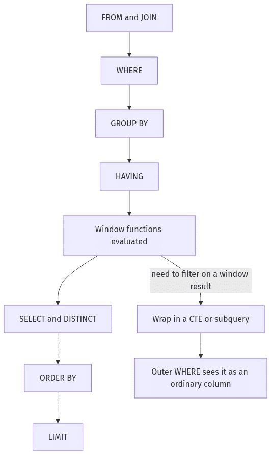
Two consequences follow directly, and both show up as Postgres errors:

SELECT name FROM employees
WHERE ROW_NUMBER() OVER (ORDER BY salary DESC) <= 3;
-- ERROR:  window functions are not allowed in WHERE

SELECT dept, COUNT(*) FROM employees GROUP BY dept
HAVING RANK() OVER (ORDER BY COUNT(*) DESC) = 1;
-- ERROR:  window functions are not allowed in HAVING

WHERE and HAVING have already finished by the time the window runs, so there is nothing for them to filter on. The corollary is more useful: because windows run after GROUP BY, a window function can take an aggregate as its argument. That is how you rank groups in one pass.

CREATE TABLE ad_events (advertiser TEXT, kind TEXT);
INSERT INTO ad_events VALUES
  ('Acme','visit'),('Acme','visit'),('Acme','visit'),('Acme','visit'),('Acme','report'),
  ('Borealis','visit'),('Borealis','visit'),('Borealis','report'),('Borealis','report'),
  ('Cinder','visit'),('Cinder','visit'),('Cinder','visit'),
  ('Cinder','visit'),('Cinder','visit'),('Cinder','visit');

SELECT advertiser,
       COUNT(*) FILTER (WHERE kind = 'visit')  AS visits,
       COUNT(*) FILTER (WHERE kind = 'report') AS reports,
       ROUND(COUNT(*) FILTER (WHERE kind='report')::numeric
             / NULLIF(COUNT(*) FILTER (WHERE kind='visit'),0), 2) AS report_rate,
       RANK() OVER (ORDER BY COUNT(*) FILTER (WHERE kind='report')::numeric
                             / NULLIF(COUNT(*) FILTER (WHERE kind='visit'),0) DESC) AS rate_rank
FROM ad_events
GROUP BY advertiser
ORDER BY rate_rank;

 advertiser | visits | reports | report_rate | rate_rank
------------+--------+---------+-------------+-----------
 Borealis   |      2 |       2 |        1.00 |         1
 Acme       |      4 |       1 |        0.25 |         2
 Cinder     |      6 |       0 |        0.00 |         3
(3 rows)

COUNT(*) FILTER (WHERE ...) is the Postgres form of a conditional count; SUM(CASE WHEN ... THEN 1 ELSE 0 END) is the portable equivalent, covered in SQL CASE WHEN and SQL COUNT.

To keep only the worst two, wrap it. The window has finished by the time the outer query's WHERE runs:

SELECT advertiser, visits, reports, report_rate
FROM (
  SELECT advertiser,
         COUNT(*) FILTER (WHERE kind='visit')  AS visits,
         COUNT(*) FILTER (WHERE kind='report') AS reports,
         ROUND(COUNT(*) FILTER (WHERE kind='report')::numeric
               / NULLIF(COUNT(*) FILTER (WHERE kind='visit'),0), 2) AS report_rate,
         RANK() OVER (ORDER BY COUNT(*) FILTER (WHERE kind='report')::numeric
                               / NULLIF(COUNT(*) FILTER (WHERE kind='visit'),0) DESC) AS rate_rank
  FROM ad_events GROUP BY advertiser
) t
WHERE rate_rank <= 2
ORDER BY rate_rank;

 advertiser | visits | reports | report_rate
------------+--------+---------+-------------
 Borealis   |      2 |       2 |        1.00
 Acme       |      4 |       1 |        0.25
(2 rows)

Snowflake, BigQuery, and Databricks add a QUALIFY clause that filters on window results without the wrapper, so the whole thing collapses to ... GROUP BY advertiser QUALIFY rate_rank <= 2. Postgres and MySQL do not have it; Postgres reports a syntax error at the window function. Know it exists, name the engine when you use it, and have the subquery form ready.

Borealis ranks first on a base of two visits. Rate metrics on tiny denominators are noise, and adding "I'd put a minimum-volume floor in the HAVING" is worth as much in an interview as the ranking itself. HAVING COUNT(*) FILTER (WHERE kind='visit') >= 1000 runs before the window, so the floor is applied to the population being ranked, which is what you want. The full clause ordering, and why moving that filter to WHERE would change the answer, is worked through in SQL Order of Operations.

Practice these on PracHub

Everything above was worked on toy tables. These are the real prompts, grouped by the pattern each one forces.

Ranking and ties

• Resolve Ties for Top-10 Users in SQL Query (Meta) — forces you to justify DENSE_RANK versus ROW_NUMBER for a fixed-size leaderboard.
• Find Top Three Books by City in Recent Months (Amazon) — aggregate units sold first, then rank inside each city, with a rolling date filter on top.
• Write SQL for social feed metrics and ties (Meta) — engagement rates across a friend graph, where the tie handling comes last and decides the answer.

Aggregate first, then rank

• Compute and rank top bad advertisers (TikTok) — a rate metric over a fixed date range, ranked and then trimmed in an outer query.
• Write complex joins and window functions (Thumbtack) — a marketplace schema where the window has to sit on top of several joins without double-counting.
• Design SQL/Pandas aggregations on retail schema (Amazon) — window logic that then has to survive translation into pandas.

Row-to-row comparisons and rolling frames

• Write rolling-window SQL over weekly cohorts (Chime) — rolling sums, week-over-week change, and an in-week rank in one query.
• Compute monthly CRR with merges and gaps (Google) — cohort retention where identity merges make "the same user" ambiguous before you can window anything.
• Write SQL and Python for transaction analytics (Robinhood) — the same windowed analysis expressed twice, which is how many DS loops are structured now.

If windows still feel shaky, the surrounding fundamentals are covered in SQL for Data Analysis and the Top 50 SQL Interview Questions. Set-operation semantics, which come up when you stack periods before windowing them, are in UNION vs UNION ALL.