MLE Knowledge Collection
Quick Overview
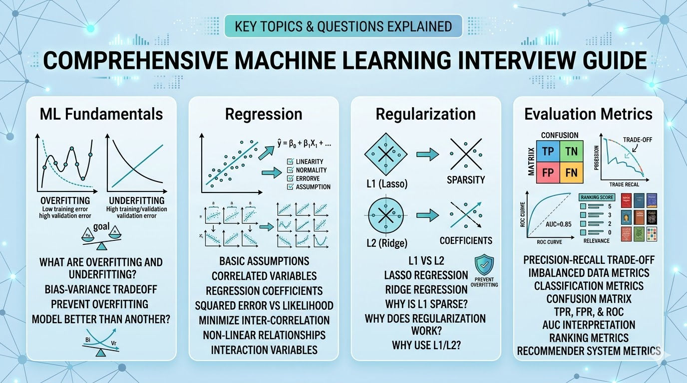
This collection covers core machine learning interview topics including ML fundamentals (overfitting and underfitting, bias–variance tradeoff), regression, regularization techniques, evaluation metrics, model comparison methods, cross-validation, and practical strategies to prevent overfitting, presented as common interview questions with detailed answers organized by topic. It is a topical Q&A study guide intended for machine learning engineers and other practitioners preparing for technical interviews or reviewing core ML concepts and evaluation methods.
A comprehensive collection of common machine learning interview questions and detailed answers, organized by topic.
Table of Contents
ML Fundamentals
1. What are Overfitting and Underfitting?
Underfitting:
- Occurs when a machine learning model is too simple to capture the underlying patterns in the data
- Model performs poorly on both training and new unseen data
- Characterized by high training and validation errors
- Solutions:
- Use more complex models
- Add more relevant features
- Reduce regularization strength
Overfitting:
- Occurs when a model becomes too complex and starts memorizing training data instead of learning generalizable patterns
- Training error is significantly lower than validation error
- Model performs poorly on new, unseen data
- Solutions:
- Reduce model complexity
- Apply regularization techniques (L1, L2, dropout)
- Use cross-validation for model selection
- Collect more training data
- Apply data augmentation
2. What is the Bias-Variance Tradeoff?
Bias:
- The difference between predicted values and the expected value of real data
- Occurs when the model oversimplifies underlying patterns and makes strong assumptions
- Leads to underfitting where the model fails to capture true relationships between features and target variables
Variance:
- Measures how spread the predicted values are from the expected value
- High variance models are sensitive to specific data points and may memorize noise or outliers
- Leads to overfitting
The Tradeoff:
- Low variance models tend to be less complex with simple structure → can lead to high bias
- Low bias models tend to be more complex with flexible structure → can lead to high variance
- Decreasing one component often increases the other
- Goal: Find the right balance between bias and variance for optimal model performance
3. What are Common Methods to Prevent Overfitting?
-
Model Complexity Reduction
- Use simpler models
- Reduce the number of parameters
-
Regularization Techniques
- L1 regularization (Lasso)
- L2 regularization (Ridge)
- Dropout (for neural networks)
- Cross-validation for model selection
-
Early Stopping
- Stop training when validation performance stops improving
-
Data-based Approaches
- Collect more training data
- Data augmentation
- Remove noisy features
4. How to Determine if One Model is Better Than Another?
Given a set of ground truths and two models:
-
Evaluation Metrics
- Choose appropriate metrics based on the problem type
- Compare performance across multiple metrics
-
Cross-Validation
- Split data into multiple folds
- Train each model on different folds and test on alternating sets
- Evaluate average performance across all folds
-
Statistical Testing
- Hypothesis testing to determine if performance differences are statistically significant
- A/B testing in production environments
-
Domain Expertise
- Consider business requirements
- Evaluate model interpretability
- Assess computational efficiency
Regression
1. What are the Basic Assumptions of Linear Regression?
-
Linearity: There is a linear relationship between independent variables (X) and dependent variable (y)
-
Independence: No relationship or correlation between the errors (residuals) of different observations
-
Normality: The residuals are normally distributed
-
Homoscedasticity: The variability of errors (residuals) is constant across all levels of independent variables
-
No Multicollinearity: Independent variables are not highly correlated with each other
2. What Happens with Correlated Variables? How to Solve?
Problems with Correlated Variables:
- Unstable coefficient estimates
- Unreliable significance tests
- Difficulties interpreting individual variable contributions
- Inflated standard errors
Solutions:
- Feature selection (remove redundant features)
- Ridge regression (L2 regularization)
- Principal Component Analysis (PCA)
- Feature engineering to create uncorrelated features
3. Explain Regression Coefficients
- Coefficients represent the change in the dependent variable associated with a one-unit change in the corresponding independent variable, while holding other variables constant
- Interpretation example: If β₁ = 2.5, then a one-unit increase in X₁ leads to a 2.5-unit increase in y, assuming all other variables remain constant
- Important: Interpretation should be done with caution and within the context of the specific model and dataset
4. Relationship Between Minimizing Squared Error and Maximizing Likelihood
- In linear regression with Gaussian error assumptions, minimizing squared error is equivalent to maximizing the likelihood of observed data
- This connection arises because the squared error can be derived from the likelihood function assuming Gaussian errors
- When Gaussian error assumptions don't hold (e.g., non-Gaussian or heteroscedastic errors), this relationship may not be valid
5. How to Minimize Inter-correlation Between Variables?
- Feature Selection: Remove highly correlated features
- PCA: Transform features into uncorrelated principal components
- Ridge Regression: Handles multicollinearity through L2 regularization
- Feature Engineering: Create new uncorrelated features from existing ones
6. Can Linear Regression Handle Non-linear Relationships?
Simple linear regression cannot accurately capture non-linear relationships, but you can:
- Add Interaction Terms: X₁ × X₂ to capture interaction effects
- Polynomial Features: Add X², X³, etc.
- Piecewise Linear Regression: Different linear models for different regions
- Transform Variables: Log, square root, or other transformations
- Switch to Non-linear Models: If relationship is strongly non-linear
7. Why Use Interaction Variables?
- Capture Non-Additive Effects: When the effect of one variable depends on another
- Improved Model Fit: Better representation of complex relationships
- Context-Specific Relationships: Model how relationships change under different conditions
- Avoid Omitted Variable Bias: Include important interaction effects
- Enhanced Interpretability: Understand how variables interact
Regularization
1. L1 vs L2 Regularization: Differences
L1 Regularization (Lasso):
- Adds the sum of absolute values of parameters to loss function
- Formula: ||β||₁ = Σ|βᵢ|
- Can shrink coefficients to exactly zero
- Produces sparse models (feature selection)
L2 Regularization (Ridge):
- Adds the sum of squared parameters to loss function
- Formula: ||β||₂ = √(Σβᵢ²)
- Shrinks coefficients towards zero but not exactly zero
- Keeps all features but with reduced impact
2. Lasso Regression
- Full name: Least Absolute Shrinkage and Selection Operator
- Objective function: L = ||ŷ - y||₂ + λ||β||₁
- Where ŷ = f_β(x) is the prediction
- Can drive coefficients to exactly zero when λ is sufficiently large
- Useful for automatic feature selection
- Creates sparse models
3. Ridge Regression
- Linear regression with L2 regularization
- Objective function: L = ||ŷ - y||₂ + λ||β||₂
- Higher λ values result in more aggressive shrinkage
- All features retained but with reduced coefficients
- Handles multicollinearity well
4. Why is L1 Sparse but L2 is Not?
- Geometric interpretation:
- L1 norm creates diamond-shaped constraint regions with corners at zero
- L2 norm creates circular (ball-shaped) constraint regions
- The optimization solution often hits the corners of the L1 diamond (where coefficients are zero)
- For L2, the solution typically hits a point on the sphere where coefficients are non-zero
- L1 penalty is not differentiable at zero, creating a "pulling" effect towards exact zeros
5. Why Does Regularization Work?
- Adds constraints to the coefficient values
- Reduces model complexity by penalizing large coefficients
- Reduces variance at the cost of slightly increased bias
- Prevents overfitting by discouraging the model from fitting noise
- Handles multicollinearity by distributing weights among correlated features
6. Why Use L1/L2 Instead of L3/L4?
- Mathematical Properties: L1 and L2 have well-studied properties that align with regularization goals
- Computational Simplicity: Higher-order norms increase complexity without significant benefits
- Interpretability: L1 (sparsity) and L2 (smoothness) have clear interpretations
- Empirical Success: L1 and L2 have proven effective in practice
- Optimization: Efficient algorithms exist for L1 and L2 regularization
Evaluation Metrics
1. Precision and Recall Trade-off
Precision:
- Measures how many positive predictions are actually true positives
- Formula: Precision = TP / (TP + FP)
- Focuses on the quality of positive predictions
- High precision = low false positives
Recall (Sensitivity):
- Measures how many actual positives are correctly identified
- Formula: Recall = TP / (TP + FN)
- Emphasizes completeness of positive predictions
- High recall = low false negatives
Trade-off:
- Improving one metric often decreases the other
- High precision, low recall: Conservative in predicting positives, few false positives but may miss true positives
- Low precision, high recall: Liberal in predicting positives, captures most true positives but generates more false positives
- Choice depends on the cost of false positives vs. false negatives
2. Metrics for Imbalanced Data
- Precision and Recall: More informative than accuracy for imbalanced datasets
- F1-Score: Harmonic mean of precision and recall, provides balanced evaluation
- Area Under Precision-Recall Curve (AUPRC): Robust to class imbalance, focuses on positive class
- ROC-AUC: Area under ROC curve, quantifies discriminative power
- Matthews Correlation Coefficient (MCC): Considers all confusion matrix elements
3. Choosing Classification Metrics
Consider:
- Problem understanding: Importance of correctly classifying each class
- Class imbalance: Use appropriate metrics for imbalanced data
- Business impact: Cost of false positives vs. false negatives
- Domain knowledge: Industry-specific requirements
- Multiple metrics: Often need to evaluate multiple aspects
4. Confusion Matrix
A table showing classification results:
- True Positives (TP): Correctly predicted positive cases
- True Negatives (TN): Correctly predicted negative cases
- False Positives (FP): Incorrectly predicted as positive
- False Negatives (FN): Incorrectly predicted as negative
From these, derive: Accuracy, Precision, Recall, F1-Score
5. TPR, FPR, and ROC
True Positive Rate (TPR):
- Also called Sensitivity or Recall
- TPR = TP / (TP + FN) = TP / (All Actual Positives)
- Measures classifier's ability to identify positive instances
False Positive Rate (FPR):
- FPR = FP / (FP + TN) = FP / (All Actual Negatives)
- Measures proportion of negatives incorrectly classified as positive
ROC Curve:
- Plots TPR vs. FPR at various classification thresholds
- Shows trade-off between sensitivity and specificity
6. AUC Interpretation
- Area Under the ROC Curve
- Represents probability that the model ranks a random positive instance higher than a random negative instance
- Range: 0 to 1
- AUC = 0.5: No better than random guessing
- AUC = 1.0: Perfect classifier
- AUC < 0.5: Worse than random (but can be inverted)
- Single number summary of model's discriminative ability
7. Ranking Metrics
Mean Reciprocal Rank (MRR):
- Formula: MRR = (1/m) × Σ(1/rankᵢ)
- Considers rank of first relevant item only
- Good when only one relevant result is expected
Recall@k:
- Formula: Recall@k = (# relevant items in top k) / (total # relevant items)
- Measures coverage of relevant items
- Challenge: Total relevant items can be very large
Precision@k:
- Formula: Precision@k = (# relevant items in top k) / k
- Measures precision of top k results
- Doesn't consider ranking quality within top k
Average Precision (AP):
- Computes average of precision@k for each relevant item
- Higher if relevant items appear earlier in list
- Considers both precision and ranking quality
Mean Average Precision (mAP):
- Average of AP across multiple queries
- Works well for binary relevance (relevant/not relevant)
Normalized Discounted Cumulative Gain (nDCG):
- DCG formula: DCGₚ = Σ(relᵢ / log₂(i+1))
- nDCG = DCG / IDCG (ideal DCG)
- Handles graded relevance scores (not just binary)
- Good for continuous relevance scores
8. Recommender System Metrics
- Precision@k: Proportion of relevant items in top k recommendations
- MRR: Good when expecting one relevant item
- mAP: For binary relevance (liked/not liked)
- nDCG: For graded relevance (ratings 1-5)
- Diversity: Average pairwise dissimilarity between recommendations
- Low similarity score = high diversity
- Important for user engagement
Choosing between metrics:
- Binary relevance → mAP
- Graded relevance → nDCG
- Single relevant item → MRR
- User experience → Include diversity metrics
Note: This guide covers fundamental concepts commonly asked in machine learning interviews. Continue practicing with real problems and stay updated with the latest developments in the field.
Comments (0)