LLM Eval Data Slicing and Debugging

What's being tested

Interviewers are checking that you can design principled analyses to find, quantify, and explain where a large language model (LLM) performs differently across inputs or populations. Expect to demonstrate experimental rigor (sample-size/power, multiplicity), metric hygiene (choice, aggregation, and calibration), and practical cohorting/slicing strategies that balance signal vs. noise. Anthropic cares because safe, robust LLMs require reproducible, interpretable failure modes — a Data Scientist must localize problems and recommend measurable remediation paths.

Core knowledge

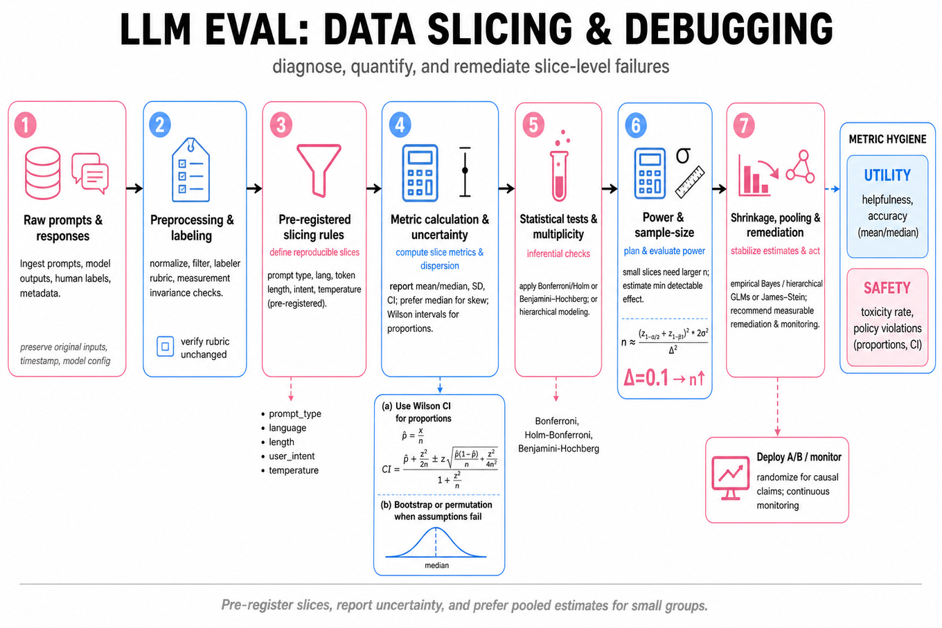
Data slicing: define slices by orthogonal, reproducible attributes (prompt type, language, token length, user intent, temperature). Prefer pre-registered slicing rules to avoid p-hacking and data snooping.
Evaluation metric hygiene: separate utility metrics (e.g., helpfulness, accuracy) from safety metrics (e.g., toxicity rate), and report both slice-level means and dispersion (SD, CI). For skewed distributions, prefer median or quantile metrics.
Uncertainty & inference: compute confidence intervals via analytic formulas when assumptions hold, otherwise use bootstrap (nonparametric) or permutation tests; for proportions, use Wilson intervals rather than Wald for small n.
Multiple comparisons: when testing many slices apply corrections (Bonferroni, Holm-Bonferroni) or control false discovery rate (Benjamini-Hochberg); alternatively use hierarchical modeling to share strength across slices.
Power & sample-size: for two-sample mean difference, approximate $n \approx \frac{(z_{1-\alpha/2}+z_{1-\beta})^2 2\sigma^2}{\Delta^2}$ where $\Delta$ is the minimum detectable effect. Small slices need much larger n or pooled analysis.
Shrinkage / Bayesian pooling: use empirical Bayes / hierarchical GLMs or James–Stein shrinkage to stabilize noisy slice estimates and reduce Type M errors (overestimation of effect sizes in small groups).
Causal vs. observational: distinguish correlation from causation; only claim causal effects if there was randomization (A/B test) or a valid identification strategy (instrument, regression discontinuity, difference-in-differences).
Anomaly diagnosis workflow: (1) verify measurement invariance (labeler rubric unchanged), (2) reproduce metric with independent data / automatic proxies, (3) slice by dimensions, (4) check time-series & rollout overlaps, (5) quantify significance and effect sizes.
Automatic vs. human labels: validate automatic proxies (ROUGE, BERTScore, embedding distances) against human ratings using confusion matrices and calibration plots (reliability diagrams); report precision/recall for binary safety labels.
Rare events & imbalanced slices: for low-prevalence safety failures use rate-per-thousand and Poisson/Negative Binomial models; for very rare outcomes prefer exact tests or aggregated buckets.
Drift & latency effects: when diagnosing temporal anomalies, use cumulative sum (CUSUM) charts or change-point detection and adjust for seasonality or backend rollouts to avoid confounding.
Practical tooling: typical analysis uses Pandas/SQL for slicing, scikit-learn / statsmodels for tests and models, and matplotlib/Altair for calibrated visualizations; pre-register analysis code and seed RNGs.

Worked example

Investigate: "Human helpfulness rating dropped 7% after a model update." First 30s framing: confirm the exact metric definition (binary vs. Likert), time window, rollout percentage, and whether labeling rubric changed. Main pillars: (1) Verify signal integrity — reproduce aggregate drop on raw logs and with independent human raters; (2) Slice by prompt attributes (language, length, intent) and by retainer cohorts (early vs. late adopters); (3) Quantify statistical evidence — compute CIs and run permutation tests per slice, correcting for multiplicity; (4) Model with a hierarchical logistic regression to estimate slice-specific effects with shrinkage. A key tradeoff: aggressively slicing can surface targeted failures but inflates false positives — prefer pre-specified slices or hierarchical modeling rather than cherry-picking. Close by proposing a targeted experiment (randomized A/B on the suspect slice) and a pre-registered analysis plan to confirm causality.

A second angle

Consider: "Calibration worsened for toxicity predictions on short prompts." The framing shifts: outcome is calibration (probabilistic), not mean helpfulness. Steps change accordingly: compute reliability diagrams and Brier score overall and per slice; use isotonic or Platt scaling diagnostics to see if miscalibration is additive or multiplicative. Because toxic events are rare on short prompts, aggregate adjacent slices or apply hierarchical Beta-binomial modeling to shrink probability estimates. Here the pragmatic recommendation might be to adjust decision thresholds for short prompts or collect targeted labeled examples, rather than retraining a full model immediately.

Common pitfalls

Pitfall: Cherry‑picked slices and uncorrected p-values — Reporting several significant slices without multiplicity correction leads to false alarms; always control FDR or use hierarchical models to temper noisy estimates.

Pitfall: Treating proxies as ground truth — Automatically computed metrics (ROUGE, embedding similarity) can misalign with human judgment; validate proxies with a confusion matrix and calibration checks before relying on them.

Pitfall: Overstating causality from observational splits — If a metric shift coincides with other operational changes (labeler pool, UI, traffic composition), avoid causal claims; propose an A/B test or quasi-experimental design instead.

Connections

Interviewers often pivot to adjacent topics: designing randomized experiments (A/B testing) to verify slice-specific hypotheses, or building monitoring that triggers when slice-level metrics cross thresholds (p99 latency-style alerts). They may also ask about labeling strategy and inter-rater reliability when human judgments are the evaluation source.