Machine Learning Model Design And Evaluation

What's being tested

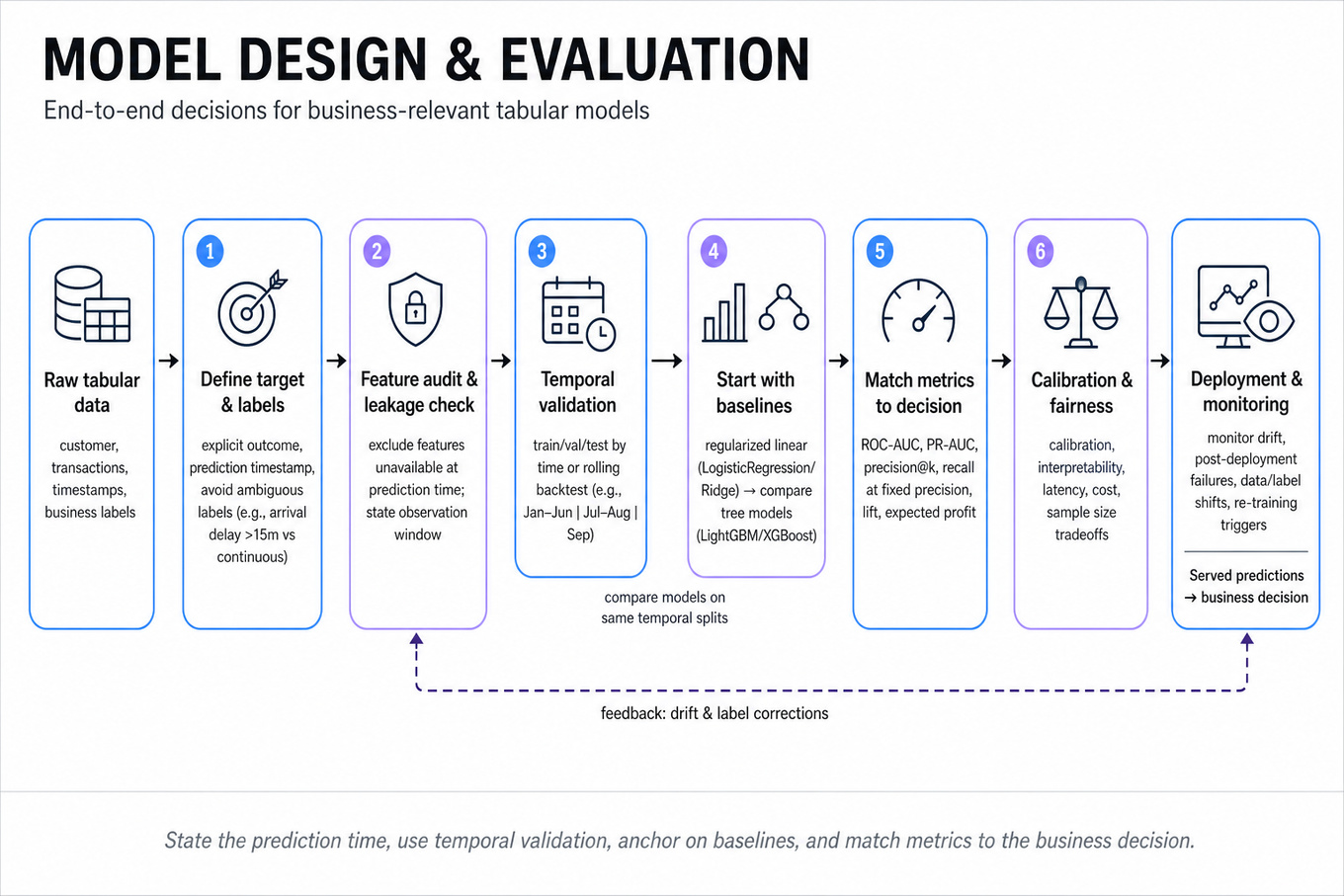
Interviewers are probing whether you can design an end-to-end predictive modeling approach for messy, business-relevant tabular problems: define the target, prevent leakage, select appropriate algorithms, evaluate with the right metric, and explain tradeoffs. For Capital One, this matters because models often influence high-stakes decisions: customer outreach, fraud operations, credit risk, servicing prioritization, and operational forecasting. A strong answer is not “use XGBoost because it performs well”; it shows disciplined thinking about time, cost, calibration, fairness, monitoring, and how offline results translate into business decisions. Expect follow-ups on why your split strategy is valid, what metric you would optimize, how you would compare models, and what could go wrong after deployment from an analytical perspective.

Core knowledge

• Target definition is the first modeling decision. For airline delays, define “delay” as arrival delay $>15$ minutes, departure delay, or continuous minutes late; for donation propensity, separate $P(\text{donate})$ from expected donation amount. Ambiguous labels create noisy evaluation and misleading business recommendations.

• Data leakage is one of the most common failure modes. Any feature unavailable at prediction time, such as actual arrival time, downstream weather updates, future donor behavior, or post-treatment campaign responses, must be excluded. Always state the prediction timestamp and feature observation window.

• Temporal validation is often better than random splitting for operational models. Use train/validation/test splits like Jan-Jun, Jul-Aug, Sep, or rolling backtests when behavior changes over time. Random splits can overstate performance when the same routes, customers, or campaigns repeat across folds.

• Baseline models anchor the conversation. Start with a simple regularized linear model such as LogisticRegression or Ridge, then compare against tree-based models like RandomForest, LightGBM, or XGBoost. A strong answer explains when interpretability, calibration, latency, sample size, and nonlinear interactions justify moving beyond the baseline.

• Classification metrics should match the decision. ROC-AUC measures ranking quality across thresholds but can look strong under heavy class imbalance. PR-AUC, precision at top $k$, recall at fixed precision, lift, and expected profit are often more relevant for rare outcomes or constrained outreach budgets.

• Regression metrics capture different costs. RMSE penalizes large errors quadratically, MAE is more robust to outliers, and quantile loss is useful when asymmetric underprediction versus overprediction costs matter. For flight delays, late extreme misses may be operationally worse than small average errors.

• Calibration matters when predicted probabilities drive policy. A model with high AUC can still produce poorly calibrated probabilities. Check reliability curves, Brier score $\text{Brier}=\frac{1}{N}\sum_i(\hat{p}_i-y_i)^2,$ and use Platt scaling or isotonic regression when probability accuracy is more important than pure ranking.

• Cost-sensitive evaluation converts model quality into business value. If contacting a donor costs $c$, expected value may be $\hat{p}_i \cdot \widehat{\text{amount}}_i - c$. For fraud or servicing workflows, define false positive and false negative costs explicitly instead of optimizing generic accuracy.

• Feature engineering for tabular DS problems usually includes time-window aggregations, categorical encodings, missingness indicators, and interaction candidates. For high-cardinality variables like airport-route pairs or merchant/customer segments, use target encoding carefully within folds to avoid leakage.

• Multicollinearity affects interpretation more than prediction for many models. In linear regression, diagnose with variance inflation factor $VIF_j=\frac{1}{1-R_j^2},$ where values above roughly 5–10 indicate instability. Tree ensembles tolerate correlated predictors better, but importance measures can become diluted or misleading.

• Hyperparameter tuning should be controlled and nested within validation. Tune max_depth, learning_rate, n_estimators, subsample, regularization, or class weights using validation folds, then report one final test result. Do not repeatedly inspect the test set; that turns it into another validation set.

• Model comparison should include uncertainty, not just leaderboard numbers. Use confidence intervals via bootstrapping, paired comparisons on the same examples, and segment-level diagnostics. A 0.003 AUC gain may not justify extra complexity if calibration, stability, or interpretability worsens.

Tip: In Capital One-style interviews, say the modeling objective and the decision objective separately. “I optimize log loss for calibrated probabilities, then choose an operating threshold based on expected profit” sounds much stronger than “I optimize accuracy.”

Worked example

For Build and evaluate airline delay prediction model, a strong first 30 seconds would clarify: “Are we predicting arrival delay or departure delay, how far before departure is the prediction made, and is the output a probability of delay or expected minutes late?” Then declare assumptions: predict whether arrival delay exceeds 15 minutes at booking time or 24 hours pre-departure, using only features known by then. Organize the answer into four pillars: target and prediction timestamp, leakage-aware features, temporal validation, and cost-sensitive evaluation. Features might include route, carrier, scheduled departure hour, day of week, seasonality, airport congestion history, and weather forecasts available before prediction time. The split should be time-based, with a final holdout month or rolling backtest to capture seasonality and operational drift. Compare a regularized logistic baseline against XGBoost or LightGBM, tracking ROC-AUC, PR-AUC, calibration, and recall at a fixed false-alert budget. A key tradeoff is classification versus regression: classification is cleaner if the business action is “flag likely delayed flights,” while regression is better if downstream planning needs expected minutes. Close by saying: “If I had more time, I’d evaluate performance by airport, carrier, route, and weather severity to find segments where the model fails or needs separate calibration.”

A second angle

For Build and evaluate donation propensity model, the same modeling discipline applies, but the objective becomes profit and treatment targeting rather than operational forecasting. The target may be whether a person donates after outreach, but a better business model often separates propensity $P(\text{donate})$ from conditional value $E[\text{amount}\mid \text{donate}]$. Random splits may be acceptable if campaigns are i.i.d., but time-based or campaign-based validation is safer when donor behavior changes seasonally. The evaluation should include expected net value, lift in the top deciles, calibration, and possibly uplift if the core decision is whom to contact rather than who would donate anyway. The main shift is causal: a high-propensity person may donate without outreach, so targeting solely on propensity can waste budget.

Common pitfalls

Pitfall: Optimizing accuracy on an imbalanced problem.

For rare delays, fraud-like events, or donation responses, a model can look “accurate” by predicting the majority class. A better answer names PR-AUC, lift, recall at fixed precision, top-$k$ capture, expected profit, or threshold-specific confusion matrices tied to the decision.

Pitfall: Treating feature availability as an implementation detail.

Saying “I would include previous delays, weather, and airport congestion” is incomplete unless you specify whether those values are known at prediction time. A stronger answer defines the prediction timestamp first, then filters features to only those observable before that timestamp.

Pitfall: Listing algorithms without model-selection logic.

A weak answer is “try logistic regression, random forest, and XGBoost and pick the best.” A stronger answer explains that logistic regression provides an interpretable calibrated baseline, tree ensembles capture nonlinearities and interactions, and final selection depends on validation performance, calibration, segment stability, and business cost.

Connections

Interviewers may pivot from model design into experimentation, especially if a propensity model leads to an outreach policy that should be A/B tested. They may also ask about causal inference, uplift modeling, fairness and bias, or model monitoring from a metric lens: drift in feature distributions, calibration decay, and segment-level performance degradation.

Further reading

• The Elements of Statistical Learning — rigorous coverage of regularization, tree methods, boosting, model assessment, and bias-variance tradeoffs.

• Interpretable Machine Learning by Christoph Molnar — practical reference for feature importance, partial dependence, SHAP-style explanations, and interpretation caveats.

• “A Few Useful Things to Know About Machine Learning” by Pedro Domingos — concise discussion of leakage, generalization, feature engineering, and practical modeling tradeoffs.