ML System Design, Recommenders, Forecasting And Allocation

What's being tested

Interviewers are probing whether you can design ML decision systems from a Data Scientist’s lens: define the prediction or causal target, choose defensible features and validation, evaluate offline and online impact, and explain tradeoffs under business constraints. The common thread is not “build a model,” but “turn messy behavioral, temporal, or operational data into a reliable decision: recommend this item, forecast this demand, allocate this courier, estimate this treatment effect.” Amazon cares because small errors in ranking, forecasting, churn prediction, and fulfillment allocation compound across millions of customers, packages, and marketplace interactions. A strong answer shows statistical discipline: avoiding leakage, validating temporally, separating prediction from causal claims, and choosing metrics aligned with customer experience and cost.

Core knowledge

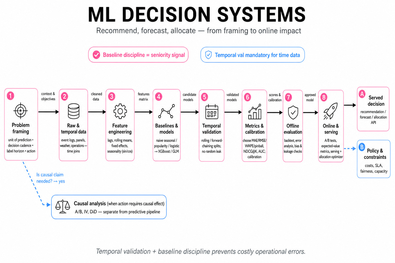
• Problem framing comes first: define the unit of prediction, decision cadence, label horizon, and action. For churn, that may be “probability a subscriber cancels in the next 30 days”; for allocation, “expected service time if courier $c$ receives package $p$ at time $t$.”

• Temporal validation is mandatory for forecasting, churn, recommendations, and logistics. Use rolling or forward-chaining splits rather than random splits: train on weeks 1–8, validate on week 9, test on week 10. Random splits leak seasonality, user lifecycle, and future availability.

• Forecasting panel data combines cross-sectional and time-series signals. For utility consumption, model household/account fixed effects, weather, holidays, lagged usage, rolling means, and seasonality terms such as $\sin(2\pi t/365)$ and $\cos(2\pi t/365)$. Compare against naive seasonal baselines before complex models.

• Baseline discipline is a major signal of seniority. For energy demand, include last-week-same-hour or same-month-last-year baselines; for recommendations, popularity and recently viewed items; for churn, logistic regression. If XGBoost beats a weak baseline only, the result is not convincing.

• Metric choice should match the decision. Regression may use MAE, RMSE, WAPE, or pinball loss; ranking may use NDCG@K, MAP@K, recall@K, and diversity; churn uses AUC, precision-recall, calibration, and lift. Cost-sensitive settings require expected value, not just accuracy.

• Calibration matters when predictions drive thresholds or optimization. A churn model with good AUC can still overstate risk; use reliability plots, Brier score, or isotonic/Platt calibration. Allocation systems need predicted durations and uncertainty, not only rank order.

• Feature leakage is the most common hidden failure. Examples: using “delivery completed timestamp” to predict package allocation, post-cancellation support contacts to predict churn, or future weather actuals in an energy forecast. Every feature should be available at decision time.

• Missing data is a signal and a risk. Distinguish MCAR, MAR, and MNAR; add missingness indicators when absence is behaviorally meaningful, impute within training folds, and avoid target-aware imputation. For subscription churn, missing billing or engagement fields may indicate disengagement.

• Double Machine Learning estimates causal effects with flexible nuisance models while reducing regularization bias. For outcome $Y$, treatment $D$, covariates $X$, residualize: $\tilde{Y}=Y-\hat{m}(X)$ and $\tilde{D}=D-\hat{e}(X)$, then estimate $\hat{\theta}=\frac{\sum_i \tilde{D}_i\tilde{Y}_i}{\sum_i \tilde{D}_i^2}.$ Use cross-fitting to avoid overfitting nuisance functions.

• Text and address-derived features can be useful but risky. TF-IDF, geohashes, learned embeddings, or parsed address components may proxy for socioeconomic status or geography. Validate representation quality, check overlap/positivity, test sensitivity to feature removal, and discuss fairness or compliance concerns.

• Recommender systems are usually staged: candidate generation, ranking, filtering, and evaluation. A DS should focus on relevance labels, negative sampling, counterfactual bias, offline metrics, segment performance, and experiment design—not low-level serving mechanics. Watch for position bias and popularity bias.

• Allocation models often combine prediction with optimization. Predict service time, failure probability, or lateness risk, then optimize an objective such as $\min \sum_{p,c} x_{pc}\hat{t}_{pc}$ subject to courier capacity, route feasibility, promised delivery windows, and fairness constraints. Evaluate both model error and operational outcomes.

Worked example

For Build a package-allocation model for couriers, start by clarifying the decision: “Are we assigning packages to couriers once per shift, continuously during the day, or at dispatch waves? Is the goal to minimize late deliveries, total route time, cost, or customer promise misses?” Then declare assumptions: each package has location, size, promised delivery window, and historical stop features; each courier has capacity, current route context, region familiarity, and shift constraints.

A strong answer can be organized into four pillars: prediction target, feature design, optimization layer, and evaluation. First, model per-stop service time or lateness probability using historical package-courier-route observations, with features like building type, delivery density, time of day, package size, weather, and courier experience in that area. Second, validate temporally and geographically, because performance on familiar neighborhoods may not generalize to new routes or seasonal peaks.

Third, feed predictions into a constrained assignment objective: minimize expected lateness or total cost while respecting capacity, route duration, promised windows, and workload balance. Fourth, evaluate offline with MAE for service time, calibration for lateness probabilities, and simulated operational metrics such as late-package rate, packages per courier hour, and customer-contact rate. The explicit tradeoff to flag is interpretability versus accuracy: a gradient-boosted model may forecast service time well, but simpler additive effects may be easier to debug when couriers or stations report implausible assignments. Close by saying: “If I had more time, I would add uncertainty-aware allocation, stress-test peak-season cohorts, and run an A/B test against the current dispatch heuristic with guardrails on late deliveries and courier workload.”

A second angle

For Apply Double ML with text-address features, the same discipline applies, but the target is causal rather than predictive. Instead of asking “Can text/address features predict the outcome?”, ask whether they adequately control confounding without violating overlap or encoding problematic proxies. The answer should frame treatment, outcome, covariates, and estimand—usually ATE or CATE—then explain cross-fitting, nuisance models for treatment and outcome, and residual-on-residual estimation. The key difference is evaluation: high predictive accuracy is insufficient; you need balance diagnostics, overlap checks, placebo tests, sensitivity analysis, and confidence intervals. Text embeddings may improve confounding control, but they can also make causal assumptions less transparent.

Common pitfalls

Pitfall: Treating every problem as a pure supervised-learning leaderboard.

A tempting answer is “I’d train XGBoost, tune hyperparameters, and optimize AUC or RMSE.” That misses the business decision. Allocation requires constraints and operational simulation; recommendations require ranking and online behavior; causal questions require identification assumptions, not just prediction.

Pitfall: Communicating a system design answer like an ML engineer.

For a Data Scientist, do not spend most of the answer on Kafka, feature-store plumbing, request fanout, or deployment topology. It is fine to mention that features must be available at decision time, but the stronger discussion is about labels, leakage, validation windows, objective functions, bias, calibration, and experiment design.

Pitfall: Ignoring segment-level and temporal failure modes.

Aggregate metrics can hide failures for new users, rural addresses, peak-season weeks, cold-start items, or high-value customers. A better answer says upfront that you would report metrics by cohort, geography, tenure, traffic source, item category, weather regime, or delivery station, depending on the product.

Connections

Interviewers may pivot from here into experimentation, especially A/B testing recommender or allocation changes with guardrail metrics like cancellation rate, late delivery rate, or customer contacts. They may also probe causal inference, time-series forecasting, ranking evaluation, fairness, or model monitoring from a metric and decision-quality perspective.

Further reading

• “Double/Debiased Machine Learning for Treatment and Structural Parameters” — Chernozhukov et al., 2018 — foundational paper for residualization, orthogonalization, and cross-fitting in causal ML.

• “Recommender Systems Handbook” — Ricci, Rokach, and Shapira — broad coverage of ranking, evaluation, cold start, and recommender tradeoffs.

• “Forecasting: Principles and Practice” — Hyndman and Athanasopoulos — practical reference for baselines, cross-validation, seasonality, and forecast accuracy metrics.