Capital One Data Scientist Interview Prep Guide

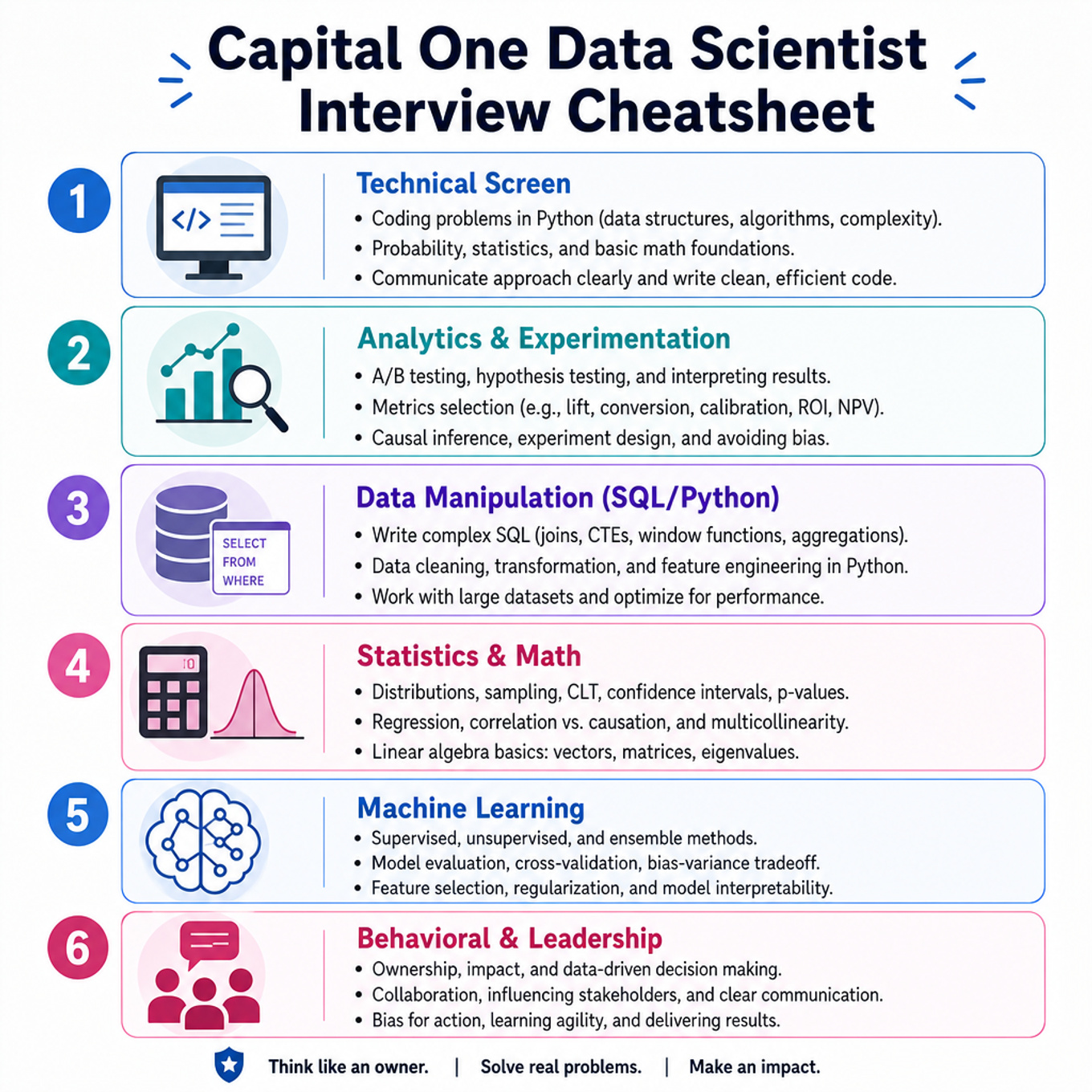
Technical Screen

Analytics & Experimentation

• A/B Testing And Causal Inference — covered in depth under Take-home Project below.

• Pricing, Demand, And Capacity Optimization — covered in depth under Onsite below.

• Product Metrics, Funnels, And Segmentation — covered in depth under Onsite below.

Data Manipulation (SQL/Python)

• SQL Analytics — covered in depth under Take-home Project below.

• Pandas Data Manipulation — covered in depth under Take-home Project below.

Statistics & Math

• Unit Economics, Break-Even, And Profit Decomposition — covered in depth under Onsite below.

• Statistical Inference, Regression, And Probability — covered in depth under Take-home Project below.

Machine Learning

• Machine Learning Model Design And Evaluation — covered in depth under Onsite below.

Behavioral & Leadership

• Behavioral Leadership And Stakeholder Communication — covered in depth under Onsite below.

Onsite

Analytics & Experimentation

• A/B Testing And Causal Inference — covered in depth under Take-home Project below.

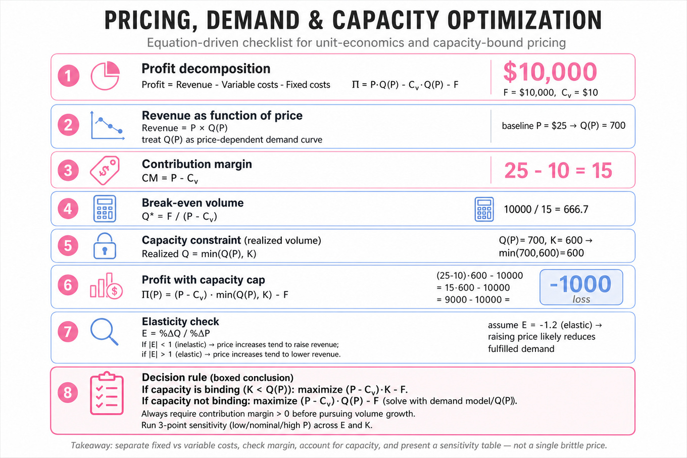
What's being tested

Interviewers are testing whether you can turn an ambiguous business scenario into a unit-economics model, identify the binding capacity constraint, and reason about pricing under uncertain demand. For a Data Scientist at Capital One, this maps directly to decisions like offer pricing, credit line utilization, acquisition incentives, servicing capacity, fraud-review queues, and profitability tradeoffs across customer segments. The interviewer is probing for structured thinking: define objective function, separate fixed vs variable costs, estimate demand response, account for constraints, and recommend a decision with sensitivity analysis rather than a single brittle number.

Core knowledge

• Profit decomposition is the foundation:
  $\text{Profit} = \text{Revenue} - \text{Variable Costs} - \text{Fixed Costs}$
  For pricing problems, write revenue as $P \times Q(P)$, where $P$ is price and $Q(P)$ is demand at that price. Always separate one-time fixed costs from per-unit marginal costs.

• Contribution margin determines whether growth helps:
  $\text{Contribution Margin} = P - C_v$
  where $C_v$ is variable cost per unit. If contribution margin is negative, selling more units worsens profit even if revenue rises. This is a common trap in surge, rent, subscription, and park-ticket problems.

• Break-even volume and break-even price are different tools. Break-even quantity is
  $Q^* = \frac{F}{P - C_v}$
  where $F$ is fixed cost. Break-even price with fixed demand is
  $P^* = C_v + \frac{F}{Q}$
  but if demand changes with price, solve $P \cdot Q(P) - C_v Q(P) - F = 0$ instead.

• Capacity constraints create discontinuities. If capacity is capped at $K$, realized volume is $\min(Q(P), K)$. The profit function becomes
  $\Pi(P) = (P - C_v)\min(Q(P), K) - F$
  This matters when a higher price reduces excess demand without lowering fulfilled volume, increasing profit and improving customer experience.

• Demand elasticity measures price sensitivity:
  $E = \frac{\%\Delta Q}{\%\Delta P}$
  If $|E| < 1$, demand is inelastic and price increases may raise revenue; if $|E| > 1$, price increases may reduce revenue. For profit, elasticity must be evaluated against margin, not revenue alone.

• Segment-level heterogeneity is often the difference between a weak and strong answer. Demand response may differ by customer segment, geography, channel, risk band, time of day, or product tier. Averages can hide profitable targeted strategies, but segmentation should be justified by sample size and business actionability.

• Optimization objective should be explicit. Common objectives include maximizing profit, maximizing revenue subject to margin constraints, maximizing customer lifetime value, minimizing unmet demand, or maintaining occupancy above a threshold. In financial services, constraints may include fairness, compliance, credit risk, operational capacity, and customer experience.

• Discrete choices require careful handling. If prices, room counts, content volumes, or staffing levels can only take integer values, do not rely solely on calculus. For small option sets, use grid search or scenario tables; for larger constrained problems, use linear programming, mixed-integer programming, or simulation-based optimization.

• Uncertainty should be modeled, not ignored. Use scenario analysis, confidence intervals, or Monte Carlo simulation when demand, costs, or conversion rates are uncertain. A strong answer reports expected profit plus downside risk, e.g., “At the recommended price, expected profit is positive, but the 10th percentile outcome is near break-even.”

• Experimentation is the cleanest way to estimate causal price effects when feasible. A randomized price or offer test can estimate demand curves, but watch for interference, seasonality, customer fairness, and long-term behavior. Use metrics like conversion_rate, average_order_value, gross_margin, retention_rate, and customer_complaints.

• Causal inference is needed when experiments are unavailable. Methods like difference-in-differences, synthetic control, propensity score weighting, or regression with fixed effects can help estimate price sensitivity from historical changes. Be clear that observational estimates are more assumption-heavy than randomized tests.

• Sensitivity analysis is not optional. Vary the highest-leverage assumptions: demand elasticity, occupancy, fixed costs, variable costs, churn, utilization, and conversion rate. A decision is stronger when you can say, “This recommendation remains profitable unless demand falls more than 18% or variable costs exceed $X.”

Worked example

For Compute profit and surge break-even price, a strong candidate would first clarify whether demand exceeds capacity, whether surge pricing changes demand, what costs are fixed versus per-service, and whether the objective is profit maximization or simply break-even. I would frame the problem as a unit-economics and capacity-constrained pricing exercise: define base demand, capacity cap, price, variable cost per fulfilled unit, and fixed cost for the period. The answer skeleton would have four pillars: calculate current profit, identify whether capacity is binding, derive the break-even surge price, and test sensitivity to demand drop from higher prices.

The key equation would be $\Pi(P) = (P - C_v)\min(Q(P), K) - F$, not just revenue minus cost using unconstrained demand. If demand is well above capacity, a modest price increase may not reduce fulfilled units, so profit rises mechanically through higher contribution margin. If demand is close to capacity, the tradeoff becomes sharper because surge pricing may reduce quantity below the cap. I would explicitly flag that treating demand as fixed under surge is a simplifying assumption and should be stress-tested with elasticity scenarios. I would close by saying that if I had more time, I’d estimate price elasticity from historical surge events or a randomized test and recommend the price that maximizes expected profit while monitoring cancellation rate and customer complaints.

A second angle

For Decide content volume and price under uncertainty, the same logic applies, but the capacity decision is made before demand is fully observed. Instead of a service cap like drivers or seats, the decision variable might be how many content units to produce, with fixed production costs and uncertain conversion or consumption. The framing shifts from break-even pricing to joint optimization: choose volume and price to maximize expected profit under demand uncertainty. A strong answer would compare conservative, base, and aggressive production scenarios, then identify where marginal expected revenue no longer exceeds marginal production cost. The interviewer is looking for whether you recognize that more content can increase demand, but also raises fixed or semi-fixed costs before revenue is guaranteed.

Common pitfalls

Pitfall: Optimizing revenue instead of profit.

A tempting answer is “raise price until revenue is maximized” or “maximize occupancy,” but neither guarantees profitability. A better answer explicitly models contribution margin, fixed costs, capacity utilization, and the possibility that lower volume at higher margin can be better than high volume at low margin.

Pitfall: Giving one number without assumptions.

Interviewers do not expect perfect real-world estimates, but they do expect transparent assumptions. If you say “the break-even price is $20” without stating demand, capacity, variable cost, and whether demand changes with price, the answer sounds mechanical rather than analytical.

Pitfall: Ignoring causal identification.

Historical correlations between price and demand are often biased because prices change during peak times, holidays, or high-demand markets. A stronger answer says how you would estimate elasticity: randomized test if feasible, otherwise quasi-experimental methods with controls for seasonality, geography, segment mix, and marketing intensity.

Connections

This topic often pivots into A/B testing, causal inference, customer segmentation, forecasting, and lifetime value modeling. For Capital One, the same reasoning can also connect to credit risk pricing, offer optimization, marketing spend allocation, fraud-review capacity, and operational queue management.

Further reading

• Pricing and Revenue Optimization by Robert Phillips — practical treatment of demand curves, capacity constraints, and revenue management.

• Mostly Harmless Econometrics by Angrist and Pischke — strong foundation for causal estimation when randomized pricing tests are not available.

• Trustworthy Online Controlled Experiments by Kohavi, Tang, and Xu — useful for designing and interpreting experiments that estimate demand and pricing effects.

Practice questions

What's being tested

Capital One is probing whether a Data Scientist can turn messy business questions into decision-grade metrics, decompose those metrics into funnels, and use segmentation to explain where performance changes come from. The interviewer is not just looking for arithmetic; they want to see whether you define a metric that matches the business objective, identify guardrails, reason about causality, and know when an apparent lift is a mix-shift artifact. This matters in financial products because small changes in conversion, pricing, risk, retention, or marketing allocation can materially change profit while also affecting fairness, compliance, and customer experience. Strong answers combine metric design, statistical validation, and clear communication of trade-offs.

Core knowledge

• Metric design starts with the decision the metric will support. A good primary metric is aligned to business value, measurable at the right unit, hard to game, and decomposable. For profit questions, use contribution profit, not raw revenue: $\text{Profit} = \text{Revenue} - \text{Variable Cost} - \text{Expected Loss} - \text{Acquisition Cost}.$

• Funnels decompose outcomes into conditional steps: exposure $\rightarrow$ click $\rightarrow$ application $\rightarrow$ approval $\rightarrow$ activation $\rightarrow$ retained customer. Overall conversion is the product of step rates: $P(\text{activation}) = P(c)\cdot P(a|c)\cdot P(appr|a)\cdot P(act|appr).$ This helps isolate whether a drop is traffic quality, UX, eligibility, pricing, or fulfillment.

• Segmentation separates heterogeneous behavior across cohorts such as channel, geography, credit band, device, product, tenure, or customer intent. Always compare both within-segment rates and segment mix; an aggregate improvement can hide declines in key groups due to Simpson’s paradox.

• Ratio metrics such as CPA, RPA, CTR, clicks per watch-minute, or profit per booking need careful denominator handling. Decide whether you need a ratio of sums, $\frac{\sum y}{\sum x}$, or an average of user-level ratios, $\frac{1}{n}\sum\frac{y_i}{x_i}$; they answer different questions and weight heavy users differently.

• Unit of analysis should match the decision. Marketing budget allocation may use channel-week or campaign-day units; customer conversion may use user-session or account units; airline profitability may use route-flight units. Mixing units creates pseudo-replication and overstates precision.

• Guardrail metrics protect against optimizing the wrong outcome. For Capital One-style decisions, guardrails might include complaint rate, delinquency, approval fairness, call-center load, fraud rate, NPS, latency, or long-term retention. A campaign that improves short-term conversion but worsens downstream loss may be value-destructive.

• Causal inference matters because segmented observational differences are rarely causal. Prefer randomized experiments when feasible; otherwise consider matched cohorts, difference-in-differences, regression adjustment, inverse propensity weighting, or instrumental variables. Be explicit about identifying assumptions such as parallel trends or no unobserved confounding.

• Experiment design should specify treatment unit, randomization level, primary metric, guardrails, minimum detectable effect, power, duration, and stopping rules. For a binary conversion metric, approximate sample size per arm scales like $n \approx \frac{2(z_{\alpha/2}+z_\beta)^2p(1-p)}{\delta^2},$ so detecting tiny lifts requires very large traffic.

• Budget allocation is a constrained optimization problem, not just ranking channels by average CPA. Use marginal return: allocate the next dollar where expected marginal profit is highest, subject to spend caps, volume constraints, and saturation. Profit per channel can be written as $\text{Profit}_j = \text{Spend}_j\left(\frac{\text{RPA}_j}{\text{CPA}_j}-1\right)$ if RPA is revenue per acquisition and CPA is cost per acquisition.

• Backtesting validates whether a metric would have made good historical decisions. For profitability metrics, test stability across time, seasonality, extreme events, and holdout periods. A metric that looks predictive only after tuning on the same time window is likely overfit.

• Anomaly diagnosis should move from metric definition to decomposition: confirm the numerator and denominator, break by funnel step, segment by major dimensions, compare to historical baselines, and inspect distributional changes rather than just means. In tools like Excel PivotTables, ensure date grouping, ISO-week logic, and tie-breaking rules are deterministic.

• Uncertainty communication is part of the answer. Report confidence intervals, practical significance, and sensitivity to assumptions, not only point estimates. For executive decisions, translate uncertainty into decision risk: “This allocation has the highest expected profit, but channel B dominates if conversion is 15% lower than estimated.”

Worked example

For Determine Optimal Budget Allocation for Maximum Profit, a strong candidate would first clarify the objective: “Are we maximizing short-term profit, lifetime value, approved accounts, or risk-adjusted contribution margin?” They would ask what data is available by channel, such as spend, inbound calls, conversion to applications, approval rate, funded account rate, revenue per acquired customer, expected loss, and operational constraints. The answer should be organized around four pillars: define the profit metric, decompose the inbound-call funnel, estimate marginal returns by channel, and recommend an allocation under constraints.

A clean skeleton might start with $\text{Expected Profit} = \text{Acquisitions}\times \text{Risk-adjusted value per acquisition} - \text{Spend}$, where acquisitions come from calls $\times$ call-to-application rate $\times$ application-to-approval rate $\times$ activation rate. Then compare channels using marginal CPA and marginal RPA, not only historical averages, because spend saturation can make the next dollar less productive than the last dollar. The candidate should explicitly flag one trade-off: reallocating budget to the channel with the best historical profit may fail if that channel has limited capacity, different customer risk, or diminishing returns at higher spend. They should also discuss validation: run a geo-level or time-split experiment if feasible, or at minimum backtest allocation rules across prior periods and perform sensitivity analysis on conversion and revenue assumptions. A strong close would be: “If I had more time, I’d estimate channel response curves with uncertainty intervals and recommend a robust allocation that performs well under conservative conversion and value assumptions.”

A second angle

For Diagnose and optimize shared workspace marketplace conversion, the same ideas apply, but the objective shifts from marketing allocation to marketplace funnel health. Instead of optimizing spend across channels, you would decompose search-to-booking conversion: visits, searches, listing views, inquiries, host responses, bookings, cancellations, and repeat usage. Segmentation becomes central because marketplace conversion may differ by city, supply density, price band, workspace type, day of week, device, and new versus returning users. The causal challenge is also different: if premium listings convert better, that may reflect location and quality rather than the effect of ranking them higher. A strong DS answer would propose experiments on ranking, pricing prompts, or inquiry flow while guarding against host response burden, cancellation rate, and supply-side fairness.

Common pitfalls

Pitfall: Optimizing a surface metric like CTR, inbound calls, or raw bookings without connecting it to downstream value.

The tempting answer is to maximize the channel with the most clicks or calls. A better answer asks whether those leads convert, whether they are profitable after risk and servicing costs, and whether the effect persists beyond the first touch.

Pitfall: Treating segmentation as proof of causality.

Saying “mobile users convert worse, so mobile causes lower conversion” is not enough. Stronger candidates frame segments as diagnostic hypotheses, then propose an experiment or quasi-experimental design to distinguish UX problems from traffic quality, customer intent, or eligibility differences.

Pitfall: Communicating only formulas and not the decision.

Interviewers want analytical rigor, but they also want a recommendation. After defining metrics and uncertainty, say what you would do: launch, hold, reallocate partially, run a powered test, or instrument more measurement before making a high-risk decision.

Connections

Interviewers may pivot from here into A/B testing, causal inference, power analysis, customer lifetime value, or model evaluation for propensity and ranking systems. They may also ask you to implement the analysis in SQL, Python, or Excel, especially aggregations, cohort tables, PivotTables, and reproducible tie-breaking for metric rankings.

Further reading

• Trustworthy Online Controlled Experiments by Kohavi, Tang, and Xu — practical reference for experiment design, metrics, guardrails, and interpretation.

• Causal Inference: The Mixtape by Scott Cunningham — accessible treatment of difference-in-differences, matching, regression discontinuity, and causal identification.

• Lean Analytics by Croll and Yoskovitz — useful product-metric framing, especially choosing metrics that match the business model and decision stage.

Practice questions

Data Manipulation (SQL/Python)

• SQL Analytics — covered in depth under Take-home Project below.

• Pandas Data Manipulation — covered in depth under Take-home Project below.

Statistics & Math

What's being tested

Capital One is testing whether you can translate a business scenario into a clean unit-economics model: revenue drivers, cost drivers, time horizon, and break-even logic. For a Data Scientist, the bar is not corporate finance depth; it is disciplined quantitative reasoning, metric definition, algebra, and the ability to explain assumptions clearly. Interviewers are probing whether you can decompose portfolio profit into customer-level components such as interchange, interest income, rewards, credit losses, operating costs, and acquisition costs. They also care whether you can distinguish accounting arithmetic from analytical judgment: what is incremental, what is fixed, what varies with customer behavior, and what uncertainty would matter before making a recommendation.

Core knowledge

• Profit decomposition starts with a simple identity:
  $\text{Profit} = \text{Revenue} - \text{Variable Costs} - \text{Fixed Costs}$
  For customer-level analysis, express everything per customer, per transaction, or per year before aggregating. Most interview mistakes come from mixing monthly and annual units.

• Unit consistency is non-negotiable. If spend is monthly, annual interchange is $12 \times \text{monthly spend} \times \text{interchange rate}$. If churn is annual, do not apply it monthly unless converted: $\text{monthly retention} \approx (1-\text{annual churn})^{1/12}$.

• Credit card revenue commonly includes interchange revenue, interest income, fees, and sometimes partner revenue. A basic formula is:
  $\text{Annual Interchange} = \text{Annual Purchase Volume} \times \text{Interchange Rate}$
  $\text{Interest Income} = \text{Revolving Balance} \times \text{APR}$
  Be ready to ask whether APR should be treated as nominal, effective, or simplified annual rate.

• Credit card costs often include rewards expense, credit losses, servicing costs, fraud losses, marketing spend, and partner payments. Rewards are usually tied to purchase volume:
  $\text{Rewards Cost} = \text{Annual Spend} \times \text{Reward Rate}$
  Credit losses are often modeled as $\text{Balance} \times \text{Loss Rate}$ or $\text{Expected Loss} = \text{PD} \times \text{LGD} \times \text{EAD}$.

• Contribution margin isolates profitability before fixed overhead:
  $\text{Contribution Margin} = \text{Revenue} - \text{Variable Costs}$
  This is often more useful than total profit when evaluating incremental customers, promotions, or pricing changes because fixed costs may not change with one more customer.

• Break-even analysis solves for the unknown that makes profit zero. If a discount costs $D$ per existing customer and each new customer contributes $M$, then:
  $\text{Break-even New Customers} = \frac{\text{Total Discount Cost}}{\text{Incremental Margin per New Customer}}$
  Use incremental margin, not gross revenue, unless costs are explicitly irrelevant.

• Customer acquisition cost or CAC should be compared against lifetime value or LTV, not just first-year profit. A simplified LTV with constant annual margin $m$, retention $r$, and discount rate $d$ is:
  $LTV = \sum_{t=1}^{T} \frac{m_t \cdot r^{t-1}}{(1+d)^t} - CAC$
  In interviews, state whether you are using first-year value or lifetime value.

• Profit margin is profit divided by revenue, not profit divided by cost:
  $\text{Profit Margin} = \frac{\text{Revenue} - \text{Cost}}{\text{Revenue}}$
  For first-year margin, include one-time acquisition or launch costs only if the question asks for first-year economics rather than steady-state economics.

• Fixed versus variable costs matter for recommendation quality. A platform cost, compliance cost, or shared servicing cost may be fixed over the relevant range; rewards, interchange network fees, credit losses, and partner revenue shares usually vary with customer behavior or balances.

• Incrementality is the Data Scientist’s edge. A promotion may attract customers who would have joined anyway, may cannibalize full-price customers, or may shift spend from another Capital One product. The relevant quantity is incremental profit:
  $\Delta \text{Profit} = \Delta \text{Revenue} - \Delta \text{Cost}$

• Segmentation often changes the answer. Transactors generate interchange but little interest; revolvers generate interest but carry higher credit risk; high-spend customers may earn more rewards expense; subprime segments may have higher expected losses. Averages can hide unprofitable cohorts.

• Sensitivity analysis is expected when inputs are uncertain. Identify the assumptions most likely to flip the decision: take rate, activation rate, average spend, revolve rate, loss rate, retention, and CAC. A strong answer says, “At the current assumptions this breaks even at X; if loss rate rises above Y, it no longer does.”

Worked example

For “Calculate Profitability and Evaluate Partnership for Credit Card Portfolio,” a strong candidate should first frame the problem as a per-customer and portfolio-level profitability model. In the first 30 seconds, ask: “Are we evaluating first-year profit or lifetime value? Are all customers active? Are spend, balances, and loss rates annual or monthly? Is the partnership cost fixed, per acquired customer, or a revenue share?” Then organize the response into four pillars: revenue, variable costs, acquisition or partnership costs, and decision criteria.

The revenue side would include annual purchase volume times interchange rate, plus revolving balances times APR if interest income is in scope. The cost side would include rewards, expected credit losses, servicing or operating costs, and any partner payment. The decision criterion should be explicit: approve the partnership if incremental LTV or expected portfolio profit is positive after CAC, not merely if revenue increases.

A tradeoff to flag is that a partner may deliver high customer volume but lower-quality or lower-activity customers, so average acquisition cost alone is insufficient. You would want cohort-level profitability by activation, spend, revolve behavior, and delinquency. Close by saying that, with more time, you would run sensitivity analysis on loss rate, retention, and activation rate, and compare partner-acquired customers to a matched baseline cohort to estimate incremental value.

A second angle

For “Calculate break-even new customers for 30% discount,” the same concept becomes a promotion break-even problem rather than a portfolio valuation problem. The key shift is that the discount may apply to existing customers, new customers, or both, so the cost base must be clarified before doing algebra. You would calculate the total margin lost from the discount, then divide by the incremental contribution margin per new customer. The Data Scientist lens is to ask whether the new customers are truly incremental or whether the promotion subsidizes customers who would have converted anyway. If conversion lift is uncertain, express the answer as a required lift or required number of incremental customers rather than a single overconfident point estimate.

Common pitfalls

Pitfall: Treating revenue as profit.

A tempting wrong answer is to use annual spend or subscription revenue as the benefit and ignore rewards, losses, servicing, and acquisition costs. A better answer decomposes gross revenue into contribution margin and only then computes profit, break-even, or payback.

Pitfall: Mixing time horizons without saying so.

Candidates often subtract a one-time CAC from monthly revenue or compare first-year profit to lifetime acquisition cost. State the horizon first: monthly, annual, first-year, or lifetime. Then convert every input to that horizon before aggregating.

Pitfall: Giving a spreadsheet answer without analytical judgment.

The interviewer does not only want arithmetic. A stronger DS answer says which assumptions are most fragile, whether the analysis should be incremental, and how customer segments could change the conclusion. For Capital One, risk-adjusted profitability matters: a high-revenue segment with high credit losses may be less attractive than a lower-revenue but stable segment.

Connections

This topic often pivots into experiment design, especially estimating whether a discount caused incremental conversion or simply subsidized existing demand. It can also connect to causal inference, cohort analysis, LTV modeling, credit-risk segmentation, and metric design for launch decisions. Be prepared to discuss how you would validate assumptions using historical cohorts, A/B tests, or matched comparisons without drifting into data pipeline architecture.

Practice questions

• Statistical Inference, Regression, And Probability — covered in depth under Take-home Project below.

Machine Learning

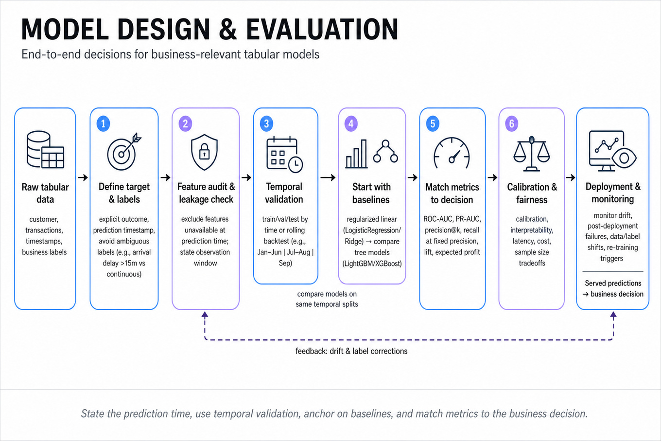
What's being tested

Interviewers are probing whether you can design an end-to-end predictive modeling approach for messy, business-relevant tabular problems: define the target, prevent leakage, select appropriate algorithms, evaluate with the right metric, and explain tradeoffs. For Capital One, this matters because models often influence high-stakes decisions: customer outreach, fraud operations, credit risk, servicing prioritization, and operational forecasting. A strong answer is not “use XGBoost because it performs well”; it shows disciplined thinking about time, cost, calibration, fairness, monitoring, and how offline results translate into business decisions. Expect follow-ups on why your split strategy is valid, what metric you would optimize, how you would compare models, and what could go wrong after deployment from an analytical perspective.

Core knowledge

• Target definition is the first modeling decision. For airline delays, define “delay” as arrival delay $>15$ minutes, departure delay, or continuous minutes late; for donation propensity, separate $P(\text{donate})$ from expected donation amount. Ambiguous labels create noisy evaluation and misleading business recommendations.

• Data leakage is one of the most common failure modes. Any feature unavailable at prediction time, such as actual arrival time, downstream weather updates, future donor behavior, or post-treatment campaign responses, must be excluded. Always state the prediction timestamp and feature observation window.

• Temporal validation is often better than random splitting for operational models. Use train/validation/test splits like Jan-Jun, Jul-Aug, Sep, or rolling backtests when behavior changes over time. Random splits can overstate performance when the same routes, customers, or campaigns repeat across folds.

• Baseline models anchor the conversation. Start with a simple regularized linear model such as LogisticRegression or Ridge, then compare against tree-based models like RandomForest, LightGBM, or XGBoost. A strong answer explains when interpretability, calibration, latency, sample size, and nonlinear interactions justify moving beyond the baseline.

• Classification metrics should match the decision. ROC-AUC measures ranking quality across thresholds but can look strong under heavy class imbalance. PR-AUC, precision at top $k$, recall at fixed precision, lift, and expected profit are often more relevant for rare outcomes or constrained outreach budgets.

• Regression metrics capture different costs. RMSE penalizes large errors quadratically, MAE is more robust to outliers, and quantile loss is useful when asymmetric underprediction versus overprediction costs matter. For flight delays, late extreme misses may be operationally worse than small average errors.

• Calibration matters when predicted probabilities drive policy. A model with high AUC can still produce poorly calibrated probabilities. Check reliability curves, Brier score $\text{Brier}=\frac{1}{N}\sum_i(\hat{p}_i-y_i)^2,$ and use Platt scaling or isotonic regression when probability accuracy is more important than pure ranking.

• Cost-sensitive evaluation converts model quality into business value. If contacting a donor costs $c$, expected value may be $\hat{p}_i \cdot \widehat{\text{amount}}_i - c$. For fraud or servicing workflows, define false positive and false negative costs explicitly instead of optimizing generic accuracy.

• Feature engineering for tabular DS problems usually includes time-window aggregations, categorical encodings, missingness indicators, and interaction candidates. For high-cardinality variables like airport-route pairs or merchant/customer segments, use target encoding carefully within folds to avoid leakage.

• Multicollinearity affects interpretation more than prediction for many models. In linear regression, diagnose with variance inflation factor $VIF_j=\frac{1}{1-R_j^2},$ where values above roughly 5–10 indicate instability. Tree ensembles tolerate correlated predictors better, but importance measures can become diluted or misleading.

• Hyperparameter tuning should be controlled and nested within validation. Tune max_depth, learning_rate, n_estimators, subsample, regularization, or class weights using validation folds, then report one final test result. Do not repeatedly inspect the test set; that turns it into another validation set.

• Model comparison should include uncertainty, not just leaderboard numbers. Use confidence intervals via bootstrapping, paired comparisons on the same examples, and segment-level diagnostics. A 0.003 AUC gain may not justify extra complexity if calibration, stability, or interpretability worsens.

Tip: In Capital One-style interviews, say the modeling objective and the decision objective separately. “I optimize log loss for calibrated probabilities, then choose an operating threshold based on expected profit” sounds much stronger than “I optimize accuracy.”

Worked example

For Build and evaluate airline delay prediction model, a strong first 30 seconds would clarify: “Are we predicting arrival delay or departure delay, how far before departure is the prediction made, and is the output a probability of delay or expected minutes late?” Then declare assumptions: predict whether arrival delay exceeds 15 minutes at booking time or 24 hours pre-departure, using only features known by then. Organize the answer into four pillars: target and prediction timestamp, leakage-aware features, temporal validation, and cost-sensitive evaluation. Features might include route, carrier, scheduled departure hour, day of week, seasonality, airport congestion history, and weather forecasts available before prediction time. The split should be time-based, with a final holdout month or rolling backtest to capture seasonality and operational drift. Compare a regularized logistic baseline against XGBoost or LightGBM, tracking ROC-AUC, PR-AUC, calibration, and recall at a fixed false-alert budget. A key tradeoff is classification versus regression: classification is cleaner if the business action is “flag likely delayed flights,” while regression is better if downstream planning needs expected minutes. Close by saying: “If I had more time, I’d evaluate performance by airport, carrier, route, and weather severity to find segments where the model fails or needs separate calibration.”

A second angle

For Build and evaluate donation propensity model, the same modeling discipline applies, but the objective becomes profit and treatment targeting rather than operational forecasting. The target may be whether a person donates after outreach, but a better business model often separates propensity $P(\text{donate})$ from conditional value $E[\text{amount}\mid \text{donate}]$. Random splits may be acceptable if campaigns are i.i.d., but time-based or campaign-based validation is safer when donor behavior changes seasonally. The evaluation should include expected net value, lift in the top deciles, calibration, and possibly uplift if the core decision is whom to contact rather than who would donate anyway. The main shift is causal: a high-propensity person may donate without outreach, so targeting solely on propensity can waste budget.

Common pitfalls

Pitfall: Optimizing accuracy on an imbalanced problem.

For rare delays, fraud-like events, or donation responses, a model can look “accurate” by predicting the majority class. A better answer names PR-AUC, lift, recall at fixed precision, top-$k$ capture, expected profit, or threshold-specific confusion matrices tied to the decision.

Pitfall: Treating feature availability as an implementation detail.

Saying “I would include previous delays, weather, and airport congestion” is incomplete unless you specify whether those values are known at prediction time. A stronger answer defines the prediction timestamp first, then filters features to only those observable before that timestamp.

Pitfall: Listing algorithms without model-selection logic.

A weak answer is “try logistic regression, random forest, and XGBoost and pick the best.” A stronger answer explains that logistic regression provides an interpretable calibrated baseline, tree ensembles capture nonlinearities and interactions, and final selection depends on validation performance, calibration, segment stability, and business cost.

Connections

Interviewers may pivot from model design into experimentation, especially if a propensity model leads to an outreach policy that should be A/B tested. They may also ask about causal inference, uplift modeling, fairness and bias, or model monitoring from a metric lens: drift in feature distributions, calibration decay, and segment-level performance degradation.

Further reading

• The Elements of Statistical Learning — rigorous coverage of regularization, tree methods, boosting, model assessment, and bias-variance tradeoffs.

• Interpretable Machine Learning by Christoph Molnar — practical reference for feature importance, partial dependence, SHAP-style explanations, and interpretation caveats.

• “A Few Useful Things to Know About Machine Learning” by Pedro Domingos — concise discussion of leakage, generalization, feature engineering, and practical modeling tradeoffs.

Practice questions

Behavioral & Leadership

What's being tested

Interviewers are probing whether you can turn ambiguous data science work into measurable business impact, communicate tradeoffs to non-technical stakeholders, and show ownership when analysis, modeling, or experimentation gets messy. For a Data Scientist at Capital One, this matters because decisions often affect customers, risk, fraud, marketing efficiency, credit outcomes, and regulatory trust—not just dashboard metrics. Strong answers show that you can define the right metric, influence partners without authority, explain uncertainty clearly, and make a defensible recommendation under constraints. The interviewer is not looking for heroic solo work; they are looking for structured judgment, stakeholder alignment, and evidence that your work changed a decision.

Core knowledge

• STAR framing is necessary but not sufficient: use Situation, Task, Action, Result, then add “Reflection.” For senior DS signals, emphasize how you scoped ambiguity, aligned stakeholders, quantified uncertainty, and changed future team behavior.

• Business impact translation should connect model or analysis outputs to financial or customer outcomes. Instead of “improved model AUC,” say “raised AUC from 0.71 to 0.78, which allowed a 12% reduction in false positives at the same approval threshold.”

• Metric design is a leadership skill. Good DS answers distinguish primary metrics, guardrail metrics, and diagnostic metrics: for example, optimizing conversion_rate while monitoring loss_rate, complaint_rate, approval_rate, model fairness slices, and customer contact frequency.

• Quantified impact should be credible, not inflated. Use a clear baseline:
  $\text{Lift} = \frac{\text{New Metric} - \text{Baseline Metric}}{\text{Baseline Metric}}$
  If attribution is uncertain, say whether the estimate came from an A/B test, backtest, difference-in-differences, or observational analysis.

• Experimental reasoning strengthens behavioral stories. Mention sample size, power, confidence intervals, and guardrails when relevant. A strong phrase: “The effect was +2.3% conversion, 95% CI [+0.8%, +3.7%], with no statistically detectable increase in downstream delinquency.”

• Causal humility matters in financial services. If you used observational data, avoid claiming causality unless the design supports it. Say “associated with,” “estimated impact,” or “directionally suggested,” and explain controls such as cohort matching, fixed effects, or sensitivity checks.

• Stakeholder segmentation improves communication. Executives usually need decision, impact, risk, and next step; product partners need metric tradeoffs and customer implications; engineering or MLE partners need feasibility, data dependencies, and evaluation criteria; compliance/risk partners need explainability and controls.

• Tradeoff communication should be explicit. Examples include precision versus recall in fraud detection, approval rate versus credit loss, personalization lift versus fairness concerns, and short-term acquisition versus long-term customer value. Show that you named the tradeoff before others had to.

• Ownership does not mean doing everything yourself. It means defining the problem, identifying gaps, unblocking decisions, escalating risks early, and creating reusable artifacts such as metric definitions, experiment readouts, model evaluation templates, or decision logs.

• Conflict resolution should be evidence-based. A strong DS answer describes competing stakeholder goals, the data you brought to the discussion, the decision rule agreed upon, and how you preserved trust even if your recommendation was not fully adopted.

• Learning orientation is evaluated through specificity. Avoid “I learned communication is important.” Better: “I now pre-align on the decision threshold before analysis, because a statistically significant result is not always operationally meaningful.”

Worked example

For “Articulate your most significant achievement,” start by framing the story in the first 30 seconds: “I’ll use an example where I led an experimentation and modeling effort to improve customer targeting while managing risk guardrails. The business goal was to increase approved applications without increasing downstream loss or adverse customer outcomes.” Clarify the role you personally played: “I owned metric design, experiment analysis, stakeholder readouts, and the recommendation; I partnered with product and risk for launch criteria.”

Organize the answer around four pillars: first, the business problem and why the existing approach was insufficient; second, the analytical approach, such as segmentation, uplift modeling, or randomized testing; third, stakeholder alignment and tradeoffs; fourth, quantified impact and what changed as a result. For example, you might say you replaced a broad campaign rule with a risk-aware segmentation strategy, evaluated it using a holdout group, and recommended rollout only for customer segments where incremental conversion exceeded expected loss.

Flag one explicit tradeoff: “The highest-response segment also had a weaker repayment profile, so I recommended excluding it from the first rollout despite the apparent short-term lift.” That sentence signals judgment beyond model optimization. Include a credible result: “The rollout improved booked accounts by 6.5% relative to control, with no measurable increase in 60-day delinquency, and reduced wasted offers by 14%.” Close with reflection: “If I had more time, I would add longer-term lifetime value tracking and pre-register the next experiment’s decision rules to reduce debate after results came in.”

A second angle

For “Deliver self-intro and justify move and company fit,” the same leadership concept becomes a concise narrative rather than a full STAR story. Your answer should connect your DS identity, the scale of problems you enjoy, and why Capital One is a logical next step. A strong framing is: “My background is in using experimentation, predictive modeling, and stakeholder-facing analytics to improve decisions in regulated or high-impact environments.” Then tie fit to Capital One’s data-driven culture, customer focus, and need for responsible decision-making in areas like credit, fraud, personalization, or digital banking. The constraint is time: in 60–90 seconds, you need one proof point, one technical strength, and one motivation—not your whole résumé.

Common pitfalls

Pitfall: Giving a task list instead of a leadership story.

A weak answer says, “I built a model, made a dashboard, and presented results.” That does not show judgment. A stronger version explains the ambiguous decision, the metric you chose, the stakeholders you aligned, the tradeoff you navigated, and the measurable outcome.

Pitfall: Overclaiming impact without a credible attribution strategy.

Saying “my model increased revenue by $10M” invites skepticism if you cannot explain the baseline, counterfactual, or experiment design. It lands better to say, “Based on the randomized holdout, we estimated$10M annualized incremental value, with sensitivity analysis showing $7M–$12M depending on adoption rate.”

Pitfall: Staying too high-level because the question is behavioral.

Behavioral does not mean non-technical. For a DS role, interviewers still expect details: metric definitions, confidence intervals, model evaluation choices, segmentation logic, or decision thresholds. The best answers are executive-readable but technically defensible when probed.

Connections

Interviewers may pivot from this topic into experiment design, metric selection, model evaluation, causal inference, or responsible AI. Be ready to explain how you would measure impact, validate a model, diagnose metric movement across cohorts, or communicate uncertainty to a senior stakeholder.

Further reading

• Trustworthy Online Controlled Experiments, Kohavi, Tang, and Xu — practical depth on experimentation, decision-making, and communicating test results.

• Storytelling with Data by Cole Nussbaumer Knaflic — useful for turning analysis into stakeholder-ready narratives.

• The Pyramid Principle by Barbara Minto — strong framework for executive communication: answer first, then support with structured evidence.

Practice questions

Take-home Project

Analytics & Experimentation

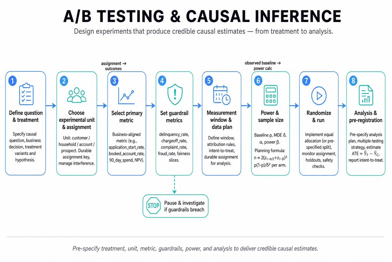
What's being tested

Capital One is probing whether you can turn a business decision into a credible causal estimate, not just report a before/after lift. For a Data Scientist, that means defining the treatment, unit of randomization, primary metric, guardrails, measurement window, power, and analysis plan before looking at results. In credit cards, marketing, and digital product changes, bad experimentation can create biased profit estimates, unfair customer outcomes, compliance risk, or over-optimistic acquisition forecasts. Strong answers show statistical rigor, business judgment, and an ability to explain tradeoffs to product, marketing, risk, and legal stakeholders without drifting into data engineering implementation details.

Core knowledge

• Randomized controlled trials estimate causal impact by making treatment independent of potential outcomes: $Y_i(1), Y_i(0)$. The target is often average treatment effect: $ATE = E[Y(1)-Y(0)]$, estimated by $\bar{Y}_T-\bar{Y}_C$ when assignment is valid.

• Experimental unit must match the decision and interference risk. For a card offer, randomize at customer, household, account, or prospect level depending on exposure sharing. If one customer can see multiple channels, define a durable assignment key and analyze by intent-to-treat.

• Primary metrics should connect to the business decision. For card acquisition, candidates include application_start_rate, approval_rate, booked_account_rate, activation_rate, 90_day_spend, net_present_value, or risk-adjusted profit. Avoid optimizing clicks if the true decision is profitable approved accounts.

• Guardrail metrics protect against harmful “wins.” In financial products, use delinquency_rate, chargeoff_rate, complaint_rate, adverse_action_rate, fraud_rate, customer_contact_rate, and fairness slices by protected-class proxies where appropriate. A campaign that increases approvals but worsens loss-adjusted margin may be a no-launch.

• Power and sample size require a baseline rate, variance, minimum detectable effect, significance level, and power. For a two-sample proportion test with equal allocation, a rough planning formula is
  $n \approx \frac{2(z_{1-\alpha/2}+z_{1-\beta})^2p(1-p)}{\delta^2}$
  per arm, where $\delta$ is the absolute MDE.

• Multiple testing matters when testing many segments, outcomes, or creative variants. Pre-register one primary metric, treat segment reads as exploratory, or adjust using Bonferroni, Holm-Bonferroni, or Benjamini-Hochberg depending on whether controlling family-wise error or false discovery rate is appropriate.

• Sequential testing is not “peek whenever and stop at $p<0.05$.” Repeated looks inflate false positives. Use fixed-horizon analysis, alpha spending, group sequential methods, or Bayesian monitoring rules agreed in advance; otherwise report results as exploratory.

• Sample ratio mismatch is a first-line validity check. If a planned 50/50 test produces 56/44 assignment, investigate targeting, eligibility, opt-outs, or logging signals before interpreting lift. The DS should diagnose from metric and assignment tables, not design event ingestion systems.

• Noncompliance and contamination are common in marketing tests. If treatment-assigned customers do not receive the offer, intent-to-treat estimates policy impact; treatment-on-the-treated may require instrumental variables using assignment as the instrument, with assumptions stated clearly.

• Variance reduction can improve sensitivity. CUPED adjusts for pre-period covariates: $Y_i^{adj}=Y_i-\theta(X_i-\bar{X})$, where $X_i$ is predictive of outcome and unaffected by treatment. Use it for spend or engagement metrics with stable pre-period behavior, not for new prospects without history.

• Causal inference without randomization requires stronger assumptions. Difference-in-differences needs parallel trends; matching or weighting needs no unobserved confounding and overlap; regression discontinuity needs no manipulation around the threshold. Always state the identification assumption and show diagnostics.

• Heterogeneous treatment effects help target policies but can overfit. Methods include causal forests, T-learners, S-learners, XGBoost, doubly robust learners, and uplift models. Evaluate with out-of-sample uplift/Qini curves, calibration by CATE decile, overlap checks, and business constraints such as fairness and adverse selection.

Worked example

For “Design A/B Test for Marketing Campaign Impact Evaluation,” a strong candidate starts by clarifying the campaign objective: incremental approved card acquisitions, incremental spend from existing cardholders, or long-term risk-adjusted profit. They would ask who is eligible, which channels are involved, whether customers can receive competing offers, and what time horizon matters for business value, such as 30-day applications and 90-day activation/spend.

The answer can be organized around four pillars: experiment design, metric framework, statistical plan, and risk/launch decision. For design, define the treatment as receiving the marketing campaign and randomize at the customer or prospect level, with a holdout control that receives business-as-usual messaging. For metrics, choose one primary metric like incremental booked_account_rate or 90_day_risk_adjusted_profit, plus funnel diagnostics such as impression_rate, click_rate, application_start_rate, approval_rate, and activation_rate.

For statistics, precompute sample size using baseline conversion and MDE, then analyze as intent-to-treat with confidence intervals and possibly logistic regression or CUPED if pre-period covariates improve precision. For risk, monitor delinquency_rate, complaints, opt-outs, and fairness slices, and define rollback criteria before launch.

A key tradeoff is whether to maximize short-term acquisitions or risk-adjusted long-term value. Optimizing approvals alone may favor applicants who are less profitable after losses, while waiting for chargeoff outcomes may take months; a practical compromise is a primary near-term metric with validated proxy guardrails. Close by saying that, with more time, you would add heterogeneous treatment effect analysis to identify which customer segments respond profitably without expanding offers to high-risk or poorly served groups.

A second angle

For “Build a causal ML pipeline end-to-end,” the same causal logic applies, but the goal shifts from estimating one average lift to learning who should receive a treatment. You would frame the estimand as CATE: $\tau(x)=E[Y(1)-Y(0)\mid X=x]$, then discuss randomized or observational training data, overlap, confounding controls, and off-policy evaluation before deployment. Instead of only asking “did the campaign work?”, the interviewer expects you to ask “for which customers does the treatment create incremental value, and how confident are we?”

The constraints are also different: policy learning can create feedback loops if high-score customers are always treated, reducing future exploration. A strong answer includes exploration holdouts, uplift calibration, sensitivity analysis, and fairness checks across customer segments. The bridge back to experimentation is that even a sophisticated causal ML model ultimately needs prospective validation through an A/B test or randomized holdout.

Common pitfalls

Pitfall: Reporting correlation as causal impact.

A tempting answer is “customers who saw the offer had 20% higher spend, so the campaign increased spend by 20%.” That ignores selection: high-value customers may have been more likely to be targeted or reachable. A better answer separates randomized assignment, actual exposure, and outcome, then states whether the estimate is intent-to-treat, treatment-on-treated, or observational with assumptions.

Pitfall: Choosing a metric that is easy instead of decision-relevant.

Click-through rate and application starts are useful diagnostics, but they are rarely sufficient for a credit-card launch decision. If the primary metric is too shallow, the test may reward misleading creative that attracts unprofitable or ineligible applicants. Tie the primary metric to incremental booked accounts, activation, spend, or risk-adjusted profit, with guardrails for credit, fraud, complaints, and fairness.

Pitfall: Sounding statistically sophisticated but operationally vague.

Interviewers do not need a lecture on every causal estimator. They want a concrete plan: unit of randomization, eligibility, treatment/control definitions, sample size, duration, metric windows, validity checks, and decision rule. Use advanced methods like doubly robust estimation or causal forests only after explaining the simpler experimental baseline and why the extra complexity is needed.

Connections

Interviewers may pivot from here into metric design, segmentation and cohort analysis, model evaluation, fairness in lending, or incrementality measurement for marketing channels. They may also ask how you would diagnose a surprising result, such as a conversion lift with worse profit, a segment reversal, or sample ratio mismatch.

Further reading

• Trustworthy Online Controlled Experiments — Kohavi, Tang, Xu — Practical experimentation design, metrics, power, variance reduction, and interpretation pitfalls.

• Causal Inference for Statistics, Social, and Biomedical Sciences — Imbens and Rubin — Rigorous potential-outcomes foundation for randomized and observational causal inference.

• Causal Inference: What If — Hernán and Robins — Free, detailed treatment of causal estimands, confounding, weighting, and longitudinal decision problems.

Practice questions

Data Manipulation (SQL/Python)

What's being tested

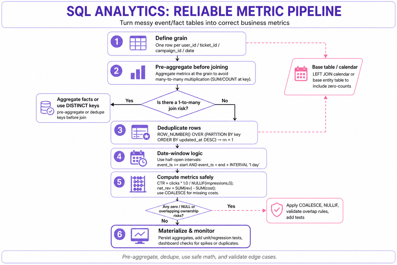
These prompts test SQL analytics: turning messy transactional or event tables into reliable business metrics using joins, filters, aggregation, deduplication, and date logic. For a Data Scientist, the bar is not just syntactically correct SQL; it is metric correctness under edge cases like duplicate rows, missing dates, zero denominators, overlapping ownership, and cost/revenue attribution.

Patterns & templates

• Grain control before joining — define one row per user_id, ticket_id, campaign_id, or date; pre-aggregate to prevent many-to-many duplication.

• Conditional aggregation with SUM(CASE WHEN ... THEN 1 ELSE 0 END) or COUNT(*) FILTER (WHERE ...) for segmented metrics in one query.

• Revenue formulas should be explicit — net revenue often means SUM(revenue) - SUM(cost); use COALESCE for missing costs or zero activity.

• Deduplication via ROW_NUMBER() OVER (PARTITION BY key ORDER BY updated_at DESC); filter rn = 1 before aggregating.

• Date-window filtering with half-open intervals like event_ts >= start_date AND event_ts < end_date + INTERVAL '1 day' to avoid timestamp boundary bugs.

• Window functions such as LAG, SUM(...) OVER, and LAST_VALUE IGNORE NULLS for forward-fill, rolling totals, and time-windowed metrics.

• Safe rate metrics use clicks * 1.0 / NULLIF(impressions, 0); never allow integer division or divide-by-zero errors in CTR.

Common pitfalls

Pitfall: Joining raw fact tables before aggregation can silently multiply revenue, visits, clicks, or donations.

Pitfall: Using COUNT(column) when nulls matter can undercount; use COUNT(*), COUNT(DISTINCT ...), or conditional counts deliberately.

Pitfall: Reporting only rows with activity misses required zero-count entities; use a base table or calendar table plus LEFT JOIN.

Practice these

The practice cards below cover the canonical variants — solve all of them and time yourself.

Practice questions

What's being tested

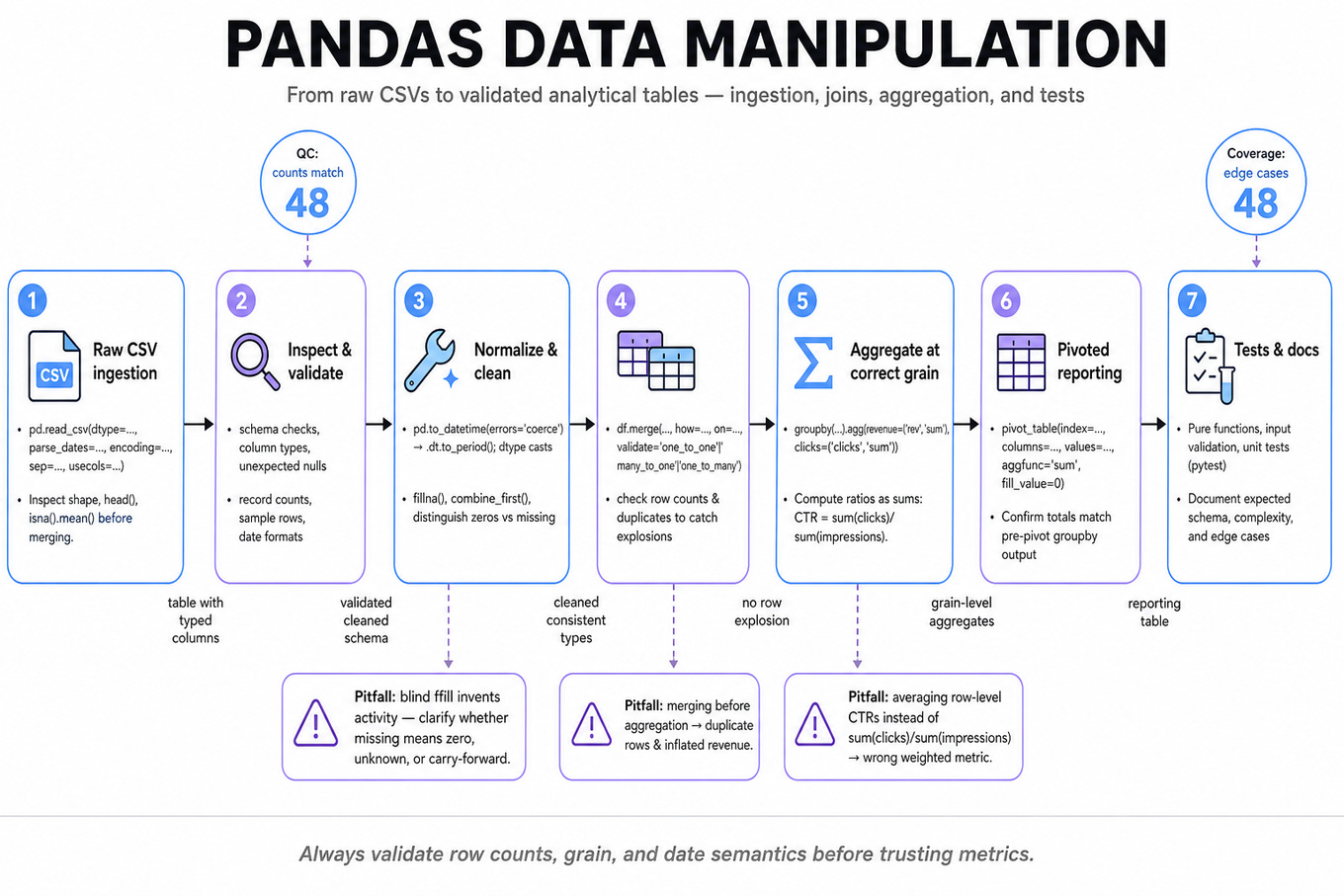
Pandas data manipulation here means turning messy local CSVs into trustworthy analytical tables: read, normalize, join, aggregate, pivot, and validate results. Interviewers are probing whether you can prevent silent analytical errors, especially duplicate joins, null mishandling, date parsing mistakes, and brittle preprocessing code.

Patterns & templates

• Robust CSV ingestion with `pd.read_csv()`: set dtype, parse_dates, encoding, sep, usecols; inspect shape, head(), isna().mean() before merging.

• Safe joins with `df.merge(..., how=..., on=..., validate=...)`: use validate='one_to_one', 'many_to_one', or 'one_to_many' to catch row explosions.

• Metric aggregation via `groupby().agg()`: compute revenue, impressions, clicks, or conversions at the correct grain before calculating ratios like CTR = clicks / impressions.

• Pivoted reporting with `pivot_table(index=..., columns=..., values=..., aggfunc='sum', fill_value=0)`: confirm totals match the pre-pivot `groupby` output.

• Date handling with `pd.to_datetime(errors='coerce')`, .dt.to_period(), `sort_values()`, and `ffill()`; always define calendar gaps versus true missing observations.

• Null and coalescing logic using `fillna()`, `combine_first()`, `where()`, and `np.select()`; distinguish missing data from valid zeros in metrics.

• Code robustness: factor transformations into pure functions, add input validation, unit-test edge cases with `pytest`, and document expected schema and complexity.

Common pitfalls

Pitfall: Merging raw fact tables before aggregation can create duplicate rows and inflate revenue, clicks, or impressions.

Pitfall: Computing CTR as the mean of row-level rates instead of sum(clicks) / sum(impressions) gives the wrong weighted metric.

Pitfall: Treating every missing date as needing `ffill()` can invent activity; clarify whether absence means zero, unknown, or carry-forward state.

Practice these

The practice cards below cover the canonical variants — solve all of them and time yourself.

Practice questions

Statistics & Math

What's being tested

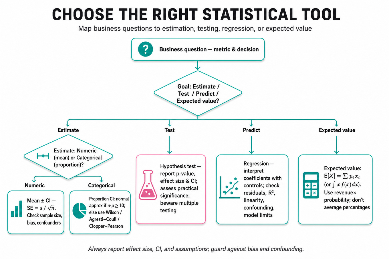
Capital One is probing whether you can turn ambiguous business or risk questions into statistical inference, probability, and decision-analysis problems with defensible assumptions. The interviewer is not just checking formula recall; they want to see whether you know when a mean, proportion, regression coefficient, confidence interval, or expected value actually answers the business question. For a Data Scientist, this matters in settings like credit policy changes, marketing tests, fraud interventions, customer segmentation, and operational metrics where decisions are made under uncertainty. Strong answers combine math correctness, interpretation in plain language, and awareness of sampling bias, confounding, multiple testing, and model limitations.

Core knowledge

• Expected value is the weighted average of possible outcomes: $E[X] = \sum_i p_i x_i$ for discrete outcomes and $E[X] = \int x f(x)\,dx$ for continuous outcomes. In profit questions, use revenue, cost, margin, and mix weights explicitly; do not average percentages unless denominators are comparable.

• Weighted averages are central when comparing customer, product, or scenario mixes: $\bar{x}_w = \frac{\sum_i w_i x_i}{\sum_i w_i}.$ A common trap is Simpson’s paradox: the aggregate metric can move opposite to every segment if the population mix changes.

• Confidence intervals estimate uncertainty around a sample statistic, usually as $\hat{\theta} \pm z_{\alpha/2}SE(\hat{\theta})$. For means, $SE(\bar{x}) = s/\sqrt{n}$; for proportions, $SE(\hat{p}) = \sqrt{\hat{p}(1-\hat{p})/n}$. Interpret a 95% interval as a procedure that covers the true parameter 95% of the time, not a 95% probability that this specific interval contains it.

• Normal approximation for proportions is reasonable when $n\hat{p} \ge 10$ and $n(1-\hat{p}) \ge 10$. For small samples or rare events, prefer the Wilson interval, Agresti-Coull interval, or exact Clopper-Pearson interval; Wilson is often a good practical default because it has better coverage without being overly conservative.

• Hypothesis testing separates the null hypothesis $H_0$ from the alternative $H_A$ and uses a p-value to quantify evidence against $H_0$. A p-value is not the probability that the null is true. Always pair it with effect size, confidence interval, and practical significance, especially for large datasets where tiny effects can be statistically significant.

• Multiple-comparison correction matters when testing many metrics, customer segments, or model features. Bonferroni correction uses $\alpha/m$ for $m$ tests and strongly controls family-wise error, but can be conservative. Benjamini-Hochberg FDR is often better when screening many hypotheses and tolerating a controlled share of false discoveries.

• Sample size and power depend on baseline rate, minimum detectable effect, variance, significance level, and desired power. For a two-sample proportion test, required $n$ grows roughly with $1/\Delta^2$, so detecting a 1% lift needs about four times as many observations as detecting a 2% lift. In interviews, state assumptions before calculating.

• Conditional probability uses $P(A \mid B) = P(A \cap B)/P(B)$, while Bayes’ theorem uses $P(A \mid B)=\frac{P(B \mid A)P(A)}{P(B)}.$ For fraud, default, approval, or churn scenarios, base rates dominate intuition: a highly accurate signal can still produce many false positives when the event is rare.

• Combinatorial probability requires matching the counting method to the sampling process: with replacement, without replacement, ordered, or unordered. Use combinations $\binom{n}{k}$ when order does not matter and permutations $P(n,k)$ when it does. Clarify independence before multiplying probabilities.

• Regression modeling estimates relationships while controlling for covariates: ordinary least squares uses $Y = X\beta + \epsilon$, while logistic regression models $\log\frac{p}{1-p} = X\beta$ for binary outcomes. In observational analysis, coefficients are associational unless identification assumptions support a causal interpretation.

• Confounding control requires including variables related to both treatment/exposure and outcome, such as seasonality, airport congestion, borrower risk tier, marketing channel, or macroeconomic conditions. Use fixed effects, interaction terms, stratification, matching, or inverse probability weighting when appropriate; avoid controlling for colliders or post-treatment variables.

• Robust uncertainty estimation is often needed in real business data. Use heteroskedasticity-robust standard errors such as HC3, clustered standard errors when observations share groups like customer, branch, or route, and bootstrap intervals with roughly 1,000–10,000 resamples when analytic standard errors are unreliable.

Worked example

For Determine Factors Influencing Airline Flight Delays Statistically, a strong candidate would first clarify the target: are we modeling whether a flight is delayed at all, delay minutes, or severe delay above a threshold such as 30 minutes? They would ask what unit of analysis is available, such as flight-level observations, and state that they will treat weather, carrier, route, airport, time of day, day of week, month, and prior-leg delay as candidate predictors. The first pillar is metric definition: binary delay suggests logistic regression, while delay minutes may need linear regression, quantile regression, or a two-part model because delay distributions are skewed and zero-inflated. The second pillar is confounding: seasonality and route mix can make an airline look worse simply because it flies more congested routes or peak-hour flights. The third pillar is uncertainty: report coefficients with confidence intervals, use robust or clustered standard errors by route or airport, and validate whether relationships are stable across time. The fourth pillar is model checking: inspect residuals, calibration for classification, out-of-time performance, and whether influential outliers dominate results. A specific tradeoff to flag is interpretability versus flexibility: a regression with airport and month fixed effects is easier to explain, while XGBoost may predict delays better but makes causal interpretation harder. The close should be: “If I had more time, I’d test interactions like weather by airport, compare out-of-sample performance, and avoid causal claims unless the design supports them.”

A second angle

For Compute optimal stopping in a die-rolling game, the same statistical discipline appears as decision-making under uncertainty rather than inference from data. Instead of estimating a parameter and confidence interval, you define states, actions, payoffs, and the expected value of continuing versus stopping. The natural method is backward induction: on the final roll, accept the value; on earlier rolls, continue only if the expected future value exceeds the current roll. This creates a threshold policy, which is the same logic a Data Scientist uses when recommending whether to approve, review, or decline a case based on expected profit or risk. The framing constraint changes: there is no sampling error if the die is fair and rules are known, but assumptions about payoff, horizon, and risk neutrality must be explicit.

Common pitfalls

Pitfall: Treating statistical significance as business significance.

A wrong-but-tempting answer is “the p-value is below 0.05, so we should act.” A stronger answer quantifies the estimated effect, confidence interval, cost of action, downside risk, and whether the magnitude matters for a business metric like expected loss, approval rate, or customer retention.

Pitfall: Ignoring denominators and mix shift.

In profit or rate comparisons, candidates often average segment percentages directly or compare aggregate means without checking segment composition. A better response computes weighted averages using transaction or customer counts, then asks whether the apparent lift is driven by true within-segment improvement or a different customer mix.

Pitfall: Jumping to a complex model before defining the estimand.

For observational regression, “I’d throw it into a random forest” can sound technically strong but misses the statistical question. If the goal is explanation or causal insight, start with the estimand, confounders, identification assumptions, and interpretable uncertainty; use flexible models as sensitivity checks or prediction benchmarks.

Connections

Interviewers may pivot from here into A/B testing, causal inference, model evaluation, or business metric design. Be ready to discuss power analysis, heterogeneous treatment effects, calibration versus discrimination, and how uncertainty affects launch or policy decisions.

Further reading

• Statistical Inference by Casella and Berger — rigorous foundation for estimators, confidence intervals, hypothesis tests, and likelihood-based reasoning.

• Data Analysis Using Regression and Multilevel/Hierarchical Models by Gelman and Hill — practical regression modeling, uncertainty, interactions, and applied interpretation.

• Trustworthy Online Controlled Experiments by Kohavi, Tang, and Xu — excellent reference for experiment design, metrics, multiple testing, and decision-making under uncertainty.

Practice questions