Statistical Inference, Regression, And Probability

What's being tested

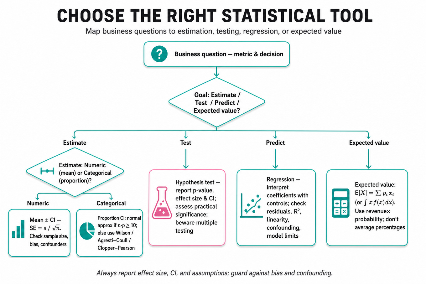
Capital One is probing whether you can turn ambiguous business or risk questions into statistical inference, probability, and decision-analysis problems with defensible assumptions. The interviewer is not just checking formula recall; they want to see whether you know when a mean, proportion, regression coefficient, confidence interval, or expected value actually answers the business question. For a Data Scientist, this matters in settings like credit policy changes, marketing tests, fraud interventions, customer segmentation, and operational metrics where decisions are made under uncertainty. Strong answers combine math correctness, interpretation in plain language, and awareness of sampling bias, confounding, multiple testing, and model limitations.

Core knowledge

• Expected value is the weighted average of possible outcomes: $E[X] = \sum_i p_i x_i$ for discrete outcomes and $E[X] = \int x f(x)\,dx$ for continuous outcomes. In profit questions, use revenue, cost, margin, and mix weights explicitly; do not average percentages unless denominators are comparable.

• Weighted averages are central when comparing customer, product, or scenario mixes: $\bar{x}_w = \frac{\sum_i w_i x_i}{\sum_i w_i}.$ A common trap is Simpson’s paradox: the aggregate metric can move opposite to every segment if the population mix changes.

• Confidence intervals estimate uncertainty around a sample statistic, usually as $\hat{\theta} \pm z_{\alpha/2}SE(\hat{\theta})$. For means, $SE(\bar{x}) = s/\sqrt{n}$; for proportions, $SE(\hat{p}) = \sqrt{\hat{p}(1-\hat{p})/n}$. Interpret a 95% interval as a procedure that covers the true parameter 95% of the time, not a 95% probability that this specific interval contains it.

• Normal approximation for proportions is reasonable when $n\hat{p} \ge 10$ and $n(1-\hat{p}) \ge 10$. For small samples or rare events, prefer the Wilson interval, Agresti-Coull interval, or exact Clopper-Pearson interval; Wilson is often a good practical default because it has better coverage without being overly conservative.

• Hypothesis testing separates the null hypothesis $H_0$ from the alternative $H_A$ and uses a p-value to quantify evidence against $H_0$. A p-value is not the probability that the null is true. Always pair it with effect size, confidence interval, and practical significance, especially for large datasets where tiny effects can be statistically significant.

• Multiple-comparison correction matters when testing many metrics, customer segments, or model features. Bonferroni correction uses $\alpha/m$ for $m$ tests and strongly controls family-wise error, but can be conservative. Benjamini-Hochberg FDR is often better when screening many hypotheses and tolerating a controlled share of false discoveries.

• Sample size and power depend on baseline rate, minimum detectable effect, variance, significance level, and desired power. For a two-sample proportion test, required $n$ grows roughly with $1/\Delta^2$, so detecting a 1% lift needs about four times as many observations as detecting a 2% lift. In interviews, state assumptions before calculating.

• Conditional probability uses $P(A \mid B) = P(A \cap B)/P(B)$, while Bayes’ theorem uses $P(A \mid B)=\frac{P(B \mid A)P(A)}{P(B)}.$ For fraud, default, approval, or churn scenarios, base rates dominate intuition: a highly accurate signal can still produce many false positives when the event is rare.

• Combinatorial probability requires matching the counting method to the sampling process: with replacement, without replacement, ordered, or unordered. Use combinations $\binom{n}{k}$ when order does not matter and permutations $P(n,k)$ when it does. Clarify independence before multiplying probabilities.

• Regression modeling estimates relationships while controlling for covariates: ordinary least squares uses $Y = X\beta + \epsilon$, while logistic regression models $\log\frac{p}{1-p} = X\beta$ for binary outcomes. In observational analysis, coefficients are associational unless identification assumptions support a causal interpretation.

• Confounding control requires including variables related to both treatment/exposure and outcome, such as seasonality, airport congestion, borrower risk tier, marketing channel, or macroeconomic conditions. Use fixed effects, interaction terms, stratification, matching, or inverse probability weighting when appropriate; avoid controlling for colliders or post-treatment variables.

• Robust uncertainty estimation is often needed in real business data. Use heteroskedasticity-robust standard errors such as HC3, clustered standard errors when observations share groups like customer, branch, or route, and bootstrap intervals with roughly 1,000–10,000 resamples when analytic standard errors are unreliable.

Worked example

For Determine Factors Influencing Airline Flight Delays Statistically, a strong candidate would first clarify the target: are we modeling whether a flight is delayed at all, delay minutes, or severe delay above a threshold such as 30 minutes? They would ask what unit of analysis is available, such as flight-level observations, and state that they will treat weather, carrier, route, airport, time of day, day of week, month, and prior-leg delay as candidate predictors. The first pillar is metric definition: binary delay suggests logistic regression, while delay minutes may need linear regression, quantile regression, or a two-part model because delay distributions are skewed and zero-inflated. The second pillar is confounding: seasonality and route mix can make an airline look worse simply because it flies more congested routes or peak-hour flights. The third pillar is uncertainty: report coefficients with confidence intervals, use robust or clustered standard errors by route or airport, and validate whether relationships are stable across time. The fourth pillar is model checking: inspect residuals, calibration for classification, out-of-time performance, and whether influential outliers dominate results. A specific tradeoff to flag is interpretability versus flexibility: a regression with airport and month fixed effects is easier to explain, while XGBoost may predict delays better but makes causal interpretation harder. The close should be: “If I had more time, I’d test interactions like weather by airport, compare out-of-sample performance, and avoid causal claims unless the design supports them.”

A second angle

For Compute optimal stopping in a die-rolling game, the same statistical discipline appears as decision-making under uncertainty rather than inference from data. Instead of estimating a parameter and confidence interval, you define states, actions, payoffs, and the expected value of continuing versus stopping. The natural method is backward induction: on the final roll, accept the value; on earlier rolls, continue only if the expected future value exceeds the current roll. This creates a threshold policy, which is the same logic a Data Scientist uses when recommending whether to approve, review, or decline a case based on expected profit or risk. The framing constraint changes: there is no sampling error if the die is fair and rules are known, but assumptions about payoff, horizon, and risk neutrality must be explicit.

Common pitfalls

Pitfall: Treating statistical significance as business significance.

A wrong-but-tempting answer is “the p-value is below 0.05, so we should act.” A stronger answer quantifies the estimated effect, confidence interval, cost of action, downside risk, and whether the magnitude matters for a business metric like expected loss, approval rate, or customer retention.

Pitfall: Ignoring denominators and mix shift.

In profit or rate comparisons, candidates often average segment percentages directly or compare aggregate means without checking segment composition. A better response computes weighted averages using transaction or customer counts, then asks whether the apparent lift is driven by true within-segment improvement or a different customer mix.

Pitfall: Jumping to a complex model before defining the estimand.

For observational regression, “I’d throw it into a random forest” can sound technically strong but misses the statistical question. If the goal is explanation or causal insight, start with the estimand, confounders, identification assumptions, and interpretable uncertainty; use flexible models as sensitivity checks or prediction benchmarks.

Connections

Interviewers may pivot from here into A/B testing, causal inference, model evaluation, or business metric design. Be ready to discuss power analysis, heterogeneous treatment effects, calibration versus discrimination, and how uncertainty affects launch or policy decisions.

Further reading

• Statistical Inference by Casella and Berger — rigorous foundation for estimators, confidence intervals, hypothesis tests, and likelihood-based reasoning.

• Data Analysis Using Regression and Multilevel/Hierarchical Models by Gelman and Hill — practical regression modeling, uncertainty, interactions, and applied interpretation.

• Trustworthy Online Controlled Experiments by Kohavi, Tang, and Xu — excellent reference for experiment design, metrics, multiple testing, and decision-making under uncertainty.