Central Limit Theorem, Confidence Intervals, And Power

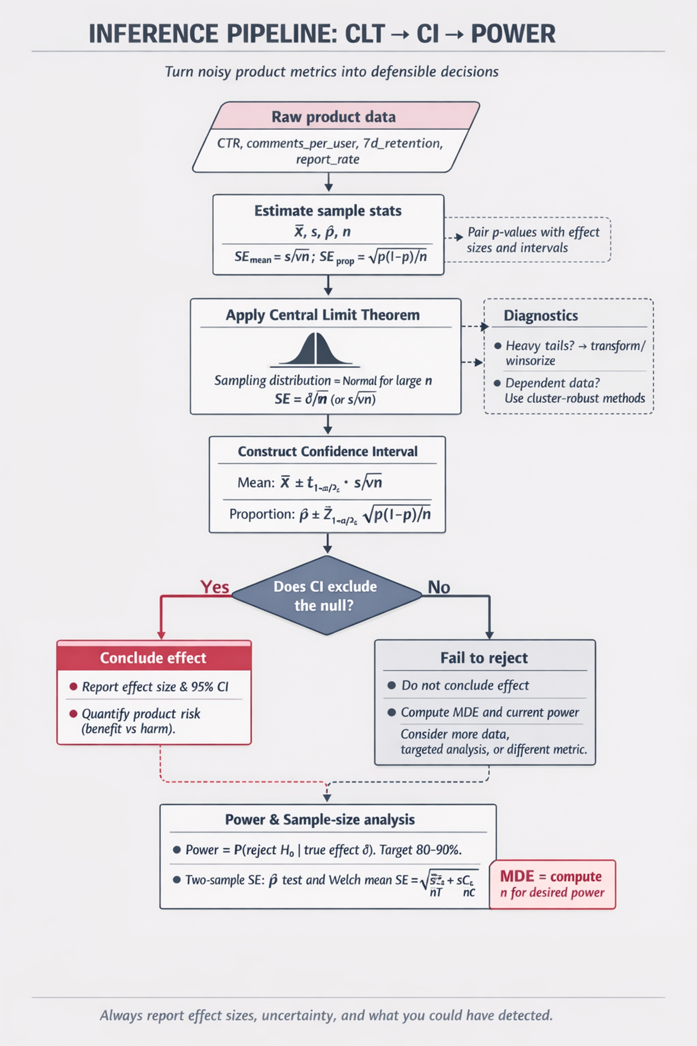
What's being tested

Interviewers are probing whether you can turn noisy product data into defensible decisions using sampling distributions, confidence intervals, hypothesis tests, and power analysis. For a Meta Data Scientist, this matters because product changes often move metrics like comments_per_user, CTR, 7d_retention, or report_rate by small amounts, and a bad inference can ship a harmful change or block a valuable one. You are expected to know the formulas, but more importantly to explain assumptions, diagnose ambiguous results, and choose an analysis plan that matches the metric and decision. Strong answers connect statistical output to product risk: “What effect sizes could we have detected, and what uncertainty remains?”

Core knowledge

• Central Limit Theorem: for sufficiently large independent samples, the sample mean $\bar X$ is approximately normal with mean $\mu$ and standard error $\sigma/\sqrt{n}$, even if the raw metric is skewed. For heavy-tailed counts like comment_count, the CLT may require large $n$ or variance-stabilizing/winsorized analyses.

• Confidence interval for a mean: when population variance is unknown, use $\bar x \pm t_{1-\alpha/2, n-1}\frac{s}{\sqrt n}.$ For large samples, $t \approx 1.96$ for a 95% interval. Interpret as “the procedure covers the true mean 95% of the time,” not “there is a 95% probability this fixed interval contains $\mu$.”

• Confidence interval for a proportion: for conversion-like metrics, $\hat p \pm z_{1-\alpha/2}\sqrt{\hat p(1-\hat p)/n}$ is common, but can be inaccurate for small $n$ or rare events. Use Wilson intervals or exact/Bayesian intervals when $\hat p$ is near 0 or 1.

• Two-sample proportion test: for comparing models or variants, test $H_0:p_1=p_2$ using $z=\frac{\hat p_1-\hat p_2}{\sqrt{\hat p(1-\hat p)(1/n_1+1/n_2)}}$ where $\hat p$ is the pooled rate under the null. For estimation, prefer an unpooled standard error for the confidence interval on $\hat p_1-\hat p_2$.

• Two-sample mean test: for metrics like comments_per_user, compare $\bar x_T-\bar x_C$ using $SE=\sqrt{s_T^2/n_T+s_C^2/n_C}.$ Use Welch’s test rather than assuming equal variance. At Meta-scale, statistical significance can occur for tiny effects, so always pair p-values with effect sizes and intervals.

• Power is $P(\text{reject }H_0 \mid \text{true effect exists})$, usually targeted at 80% or 90%. For a two-sided two-sample proportion test with equal allocation, approximate per-arm sample size is $n \approx \frac{2(z_{1-\alpha/2}+z_{1-\beta})^2p(1-p)}{\delta^2}$ where $\delta$ is the minimum detectable effect in absolute rate points.

• Minimum detectable effect: the MDE should be product-relevant, not just mathematically convenient. If baseline CTR is 10%, an absolute lift of 0.1 percentage points is a 1% relative lift; clarify whether stakeholders mean absolute or relative effects.

• Type I and Type II errors: $\alpha$ is false-positive risk; $\beta$ is false-negative risk. Lowering $\alpha$ or increasing power requires more sample size. A non-significant result does not prove no effect; it often means the confidence interval still includes meaningful positive and negative effects.

• Multiple testing correction: testing many metrics, segments, or model variants inflates false positives. Bonferroni correction controls family-wise error using $\alpha/m$ and is conservative; Benjamini–Hochberg controls false discovery rate and is often more powerful for many exploratory metrics.

• Sequential monitoring: repeatedly peeking at p-values without adjustment increases false positives. If interim looks are planned, use designs such as O’Brien–Fleming boundaries, alpha spending, or always-valid inference. In an interview, explicitly say whether the test duration and decision rule were fixed before observing results.

• Variance misspecification: underestimating variance makes sample-size plans too optimistic and confidence intervals too narrow. Product metrics often have user-level clustering, seasonality, and heavy users; compute variance at the randomization unit, typically user-level, rather than treating events as independent.

• Decision quality under uncertainty: statistical significance is not the only launch criterion. A small positive but non-significant result may be worth further testing if upside is high and risk is low; a significant lift in engagement may still be blocked if guardrails like hide_rate, unfollow_rate, or integrity_report_rate worsen.

Worked example

For “Construct a 95% Confidence Interval for Comment Counts”, a strong candidate first clarifies the unit of analysis: “Are these comments per user, per post, or per session, and is the sample randomly drawn from the target population?” They would also ask whether extreme users or bots are included, because comment counts are often skewed and overdispersed. The answer skeleton should have four pillars: define the estimand, compute the sample mean and standard error, choose the appropriate critical value, and interpret the interval in product language.

A concise framing could be: “Assuming we have $n$ independent users with comment counts $x_i$, I estimate the population mean with $\bar x$ and uncertainty with $s/\sqrt n$.” Then construct $\bar x \pm 1.96s/\sqrt n$ for a large sample, or use a $t$ critical value for smaller samples. The candidate should explicitly flag that the CLT applies to the sample mean, not the raw comment distribution; the raw counts can be highly non-normal while the mean is still approximately normal at large $n$. A useful tradeoff to mention is whether to use the raw mean, a winsorized mean, or a bootstrap interval if a few outliers dominate variance. Close by saying: “If I had more time, I’d inspect the distribution by cohort, check independence at the user level, and compare the normal-theory interval with a bootstrap interval for robustness.”

A second angle

For “Diagnose a non-significant experiment outcome”, the same statistical concepts apply, but the task shifts from computation to decision diagnosis. Instead of simply saying “p > 0.05, so no effect,” a strong answer asks whether the experiment was powered for the observed effect size and whether the confidence interval rules out practically meaningful lifts or harms. If the interval is wide, the result is inconclusive; if it is narrow around zero, the product effect is likely small. The candidate should also consider variance inflation, sample-ratio mismatch, novelty effects, segment heterogeneity, and guardrail metrics. The key transfer is that uncertainty quantification drives the decision, not the binary significance label.

Common pitfalls

Pitfall: Treating the p-value as the probability the null hypothesis is true.

A wrong-but-tempting answer is “p = 0.03 means there is a 97% chance the treatment works.” A better answer is: “If there were truly no effect and assumptions hold, we would see a result this extreme or more extreme 3% of the time.” Then translate that into a decision using effect size, confidence interval, and business risk.

Pitfall: Ignoring the unit of randomization and independence.

If users are randomized but you analyze impressions as independent rows, the standard error can be badly understated because one user can generate many correlated events. For Meta-style experiments, aggregate to the user or randomization unit first, then compare user-level outcomes unless you have a valid clustered variance estimator.

Pitfall: Communicating only formulas without product interpretation.

An interviewer is not satisfied by “use $1.96 \times SE$” if you cannot say what the interval means for launch. State whether the plausible effect range includes meaningful harm, meaningful upside, or only negligible differences; then recommend ship, do not ship, ramp, or collect more data based on that uncertainty.

Connections

Expect pivots into A/B testing, causal inference, metric design, multiple comparisons, and Bayesian experimentation. Interviewers may also connect power and confidence intervals to ranking-model evaluation, where offline metric lifts like NDCG or AUC need uncertainty estimates before deciding whether to run an online test.

Further reading

• Trustworthy Online Controlled Experiments by Kohavi, Tang, and Xu — practical treatment of experiment design, metrics, variance, peeking, and decision-making.

• Statistical Power Analysis for the Behavioral Sciences by Jacob Cohen — classic reference for effect sizes, power, and sample-size reasoning.

• The American Statistician: “Moving to a World Beyond p < 0.05” — useful perspective on avoiding binary significance thinking.