Model Telemetry And Inference Cost Analytics

What's being tested

The interviewer is probing your ability to treat model telemetry as measurable, testable signals: define robust metrics, detect and diagnose regressions, and quantify trade-offs between inference cost and model quality. They want to see statistical rigor (power, CIs, hypothesis framing), segmentation and causal reasoning (is cost change due to inputs, routing, or model change?), and pragmatic decisions for what to instrument and act upon at scale. OpenAI cares because inference costs are economically material and can interact with user experience in subtle, segment-specific ways.

Core knowledge

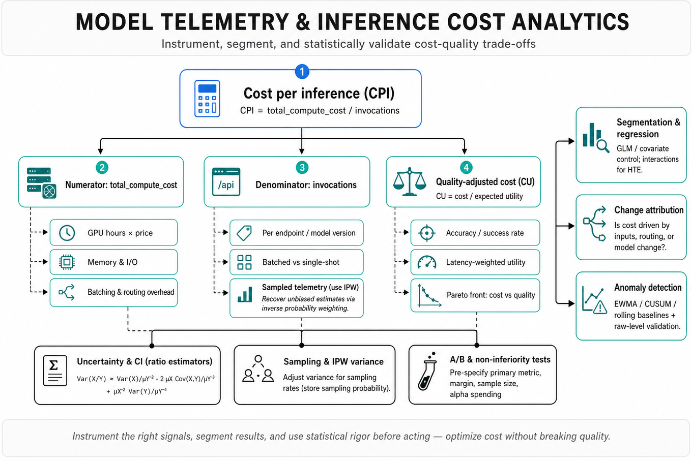
Cost per inference basics: compute as $\text{CPI} = \frac{\text{total\_compute\_cost}}{\text{invocations}}$ and track aggregated and segmented CPI (by model version, endpoint, region, client).
Latency distribution vs mean: track p50, p90, p99 (use quantile sketches like t-digest for streaming). Heavy tails can dominate cost and user experience despite benign means.
Quality-cost tradeoff: evaluate cost-effectiveness via cost per correct prediction or cost-weighted utility: $\text{CU}=\frac{\text{cost}}{\text{expected utility}}$ and compare Pareto fronts across model variants.
Ratio estimators & Delta method: for CPI or cost-per-success ratios, estimate variance with the delta method: $\text{Var}(\tfrac{X}{Y})\approx \frac{\text{Var}(X)}{\mu_Y^2} - 2\frac{\mu_X\text{Cov}(X,Y)}{\mu_Y^3} + \frac{\mu_X^2\text{Var}(Y)}{\mu_Y^4}$ for CI construction.
Sampling and weighting: when telemetry is sampled, use inverse probability weighting (IPW) to recover unbiased estimates; ensure you know sampling rates and include them in variance estimates.
A/B and non-inferiority tests: design tests with primary metric (e.g., accuracy, latency cost), choose margins for non-inferiority, compute sample size with variance estimates and desired power, and plan pre-specified stopping rules (alpha spending).
Attribution via segmentation/regression: use stratified analyses and linear/GLM regressions with covariates (features, client, region, time-of-day) to control confounding when attributing cost changes. Consider interactions for heterogeneous treatment effects.
Anomaly detection from a metric lens: detect change-points in aggregated metrics using rolling baselines, EWMA, or CUSUM with seasonality adjustments; validate with raw-level sampling to avoid false positives from aggregation artifacts.
Micro vs macro telemetry: combine aggregated daily metrics (BigQuery, Postgres) with sampled request traces (Prometheus, logs) for debugging; treat traces as diagnostic samples, not population estimates unless sampling is known.
Instrumentation for causal tests: prefer randomized assignment (A/B) to estimate causal cost impacts of model changes; where randomization is impossible, use difference-in-differences or instrumental variables with careful assumptions.
Cost allocation & amortization: when GPU/CPU billing is per-hour, amortize cost across invocations using measured utilization (e.g., GPU-seconds) rather than wall-clock machine-hours to avoid misleading per-request CPI.
Power & HTE planning: compute detectable effect sizes per segment; if small segments drive high costs, plan for targeted experiments or sequential buckets instead of one global test.

Worked example — "Investigate a sudden increase in inference cost while accuracy unchanged"

First 30s: clarify the signal (which cost metric rose? aggregated CPI, p99 latency, or GPU-hours?) and scope (single model version, region, or client subset), and ask about recent deploys or config changes. Skeleton approach: (1) validate telemetry and sampling rates, (2) segment by version/region/client/time and compute delta-CPI with CIs, (3) inspect request-level traces to find tail events, input-size shifts, or cache misses, (4) run regression to attribute cost to covariates (input length, prompt type, model routing), (5) simulate what-if: re-score historical requests against old/new model to confirm. A key tradeoff to highlight: full re-processing of historical traffic (gold standard) is accurate but expensive and slow; a targeted sample or cohort replay gives fast, lower-cost signals. Close by proposing immediate mitigations (roll back a suspect change, throttle expensive routes) and next steps: instrument finer-grained compute metrics and run an A/B to isolate cause.

A second angle — "Design an experiment to evaluate a lower-cost model variant"

Frame primary and secondary metrics up-front: a primary quality metric (e.g., task-specific accuracy or user engagement), and a primary cost metric (e.g., CPI or cost-per-success). Choose test type: non-inferiority if tolerating small quality drops for cost savings. Compute sample size using anticipated variance of the quality metric and the chosen non-inferiority margin; when cost is noisy, use stratified randomization by high-cost segments to ensure balance. Plan for heterogeneous treatment effects: predefine segment analyses, and adjust for multiple comparisons. Operational considerations: synchronous vs async routing, guardrails for high-cost outliers, and predefined interim analyses with alpha-spending to allow early stop for clear wins or losses.

Common pitfalls

Pitfall: trusting global means without checking tails.
If you report only average latency or CPI, you will miss rare, high-cost requests that can dominate billing or cause outages; always report p99/p999 and show distributional plots.

Pitfall: forgetting sampling design in metrics.
Telemetry traces are often sampled; treating trace-derived averages as population estimates yields biased CPI — always account for sampling probability with IPW and carry sampling uncertainty into CIs.

Pitfall: answering "why" with correlation not causation.
Pointing to input changes after a deploy is tempting, but without randomization or causal identification you must label findings as associative and propose causal checks (A/B, replay, IV) rather than assert direct attribution.

Connections

This topic naturally pivots to experimentation design (power, sequential testing), model evaluation (calibration, utility-weighted metrics), and anomaly detection for operational metrics. Interviewers may ask to expand into segmentation/Heterogeneous Treatment Effects or cost-aware optimization (constrained model training/pruning).