Personalization, Collaborative Filtering, And Bandits

What's being tested

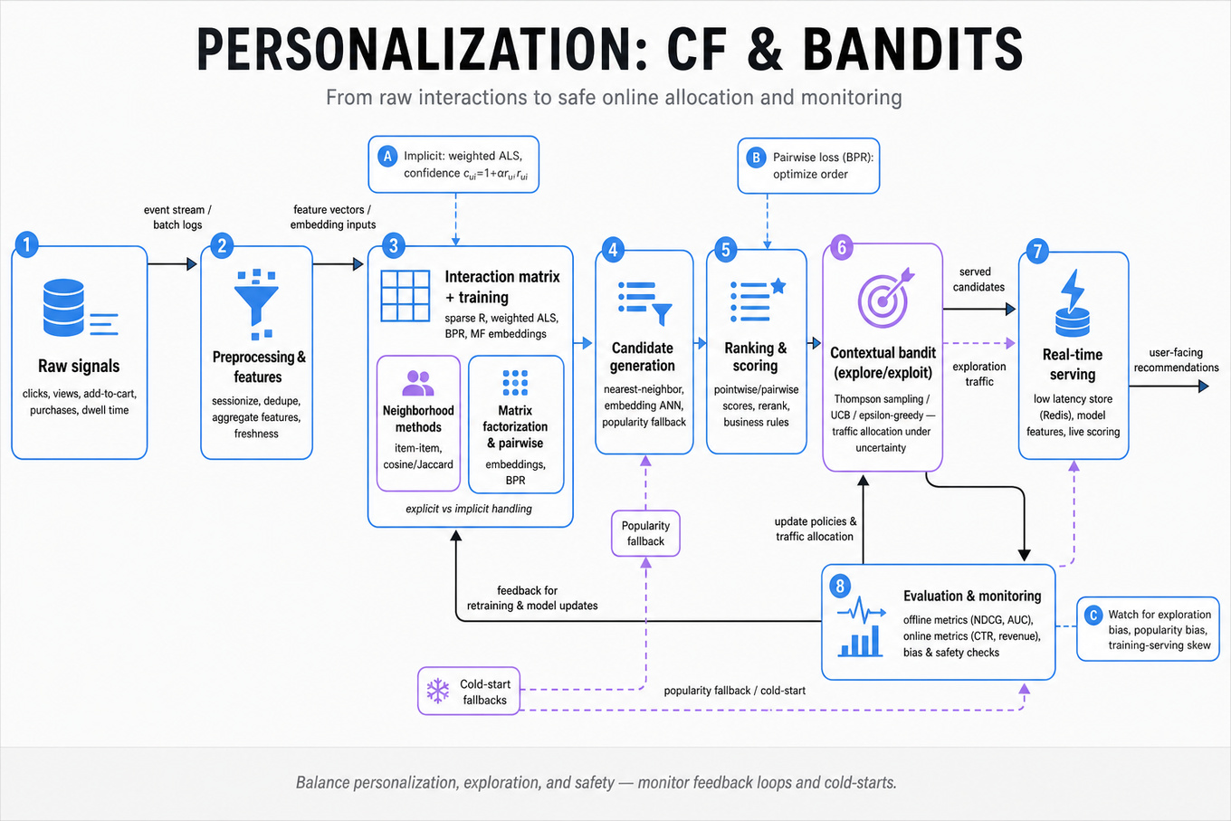
Interviewers are probing whether you can explain personalized recommendation methods at both the modeling and production levels: how collaborative filtering learns user–item affinity, how bandits allocate traffic under uncertainty, and how these methods are evaluated and served safely. For an Amazon Machine Learning Engineer, this matters because recommendations, ads, search ranking, merchandising, and content placement all require scalable personalization under latency, freshness, cold-start, and feedback-loop constraints. You should be able to compare algorithms, state modeling assumptions, discuss offline versus online evaluation, and identify deployment risks like exploration bias, popularity bias, and training-serving skew.

Core knowledge

• Collaborative filtering assumes users with similar historical behavior will prefer similar items. The core signal is a sparse user–item interaction matrix $R \in \mathbb{R}^{m \times n}$, where entries may represent ratings, purchases, clicks, views, dwell time, or add-to-cart events.

• Neighborhood-based methods compute similarity between users or items, then recommend based on nearest neighbors. Item-item collaborative filtering is often more stable than user-user filtering because item relationships change more slowly; similarity can use cosine, Jaccard, Pearson correlation, or adjusted cosine.

• Matrix factorization represents each user and item with latent vectors:
  $\hat r_{ui} = p_u^\top q_i + b_u + b_i + \mu$
  where $p_u$ and $q_i$ are embeddings, $b_u$ and $b_i$ are biases, and $\mu$ is the global mean. This scales better than neighborhood methods for large sparse matrices.

• Explicit feedback uses ratings or thumbs-up signals and often optimizes squared error, but ratings are sparse and biased toward highly engaged users. Implicit feedback uses clicks, purchases, views, or streams; missing entries are not true negatives, so methods like weighted ALS use confidence $c_{ui}=1+\alpha r_{ui}$.

• Pointwise losses predict an absolute label such as click probability or rating. Pairwise losses, such as Bayesian Personalized Ranking (BPR), optimize relative ordering: a user should rank an observed item above an unobserved one, often with loss $-\log \sigma(\hat r_{ui} - \hat r_{uj})$.

• Cold start is a central production issue. New users need contextual, demographic, query, session, or popularity-based fallbacks; new items need content features, catalog metadata, image/text embeddings, or exploration traffic before collaborative signals accumulate.

• Approximate nearest neighbor retrieval is common for candidate generation from learned embeddings. Systems often use `FAISS`, `ScaNN`, or `Annoy` to retrieve top-K candidates under millisecond-level latency, then send them to a heavier ranker.

• Bandit algorithms address the exploration–exploitation tradeoff: exploiting known high-performing actions maximizes short-term reward, while exploring uncertain actions improves future decisions. Regret is commonly defined as $R_T = T\mu^\* - \sum_{t=1}^{T} r_t$.

• Epsilon-greedy chooses the current best arm with probability $1-\epsilon$ and explores randomly with probability $\epsilon$. It is simple and production-friendly, but uniform exploration can waste traffic on clearly poor arms unless $\epsilon$ decays or arms are filtered.

• Upper Confidence Bound (UCB) chooses actions using optimism under uncertainty, for example:
  $a_t = \arg\max_a \left(\hat\mu_a + c\sqrt{\frac{\log t}{N_a}}\right)$
  It naturally explores under-sampled arms, but assumes reward estimates and confidence terms are meaningful and comparable.

• Thompson sampling samples from each arm’s posterior distribution and chooses the arm with the highest sampled reward. For Bernoulli rewards, a common model is `Beta(alpha, beta)` per arm; it often performs well in practice and handles uncertainty more smoothly than deterministic UCB.

• Contextual bandits condition action choice on features such as user, item, query, device, time, and session context. Production implementations may use linear models, gradient-boosted trees, or neural rankers, but must log propensities to support unbiased offline evaluation via inverse propensity scoring.

Worked example

For Explain Collaborative Filtering Approaches, a strong candidate should first frame the problem: “Are we recommending products, videos, or ads; do we have explicit ratings or implicit events; and is the goal candidate generation, ranking, or both?” Then declare assumptions: “I’ll assume a large sparse user–item matrix with implicit feedback such as clicks and purchases, and a latency-sensitive serving path.” A clean answer has four pillars: neighborhood methods, matrix factorization, implicit-feedback modeling, and production considerations.

Start with neighborhood methods because they are intuitive: user-user similarity recommends what similar users liked, while item-item similarity recommends items co-consumed with items the user interacted with. Then move to matrix factorization: learn user and item embeddings using ALS, SGD, or BPR, and score with a dot product. For implicit feedback, emphasize that unobserved does not mean disliked; weighted ALS or sampled negatives are better than treating every missing cell as a zero.

The tradeoff to flag explicitly is interpretability and simplicity versus scalability and representation power. Item-item models are easy to debug and cache, while factorization models handle sparsity better and produce embeddings usable in `FAISS`-style retrieval. Close by saying: “If I had more time, I would discuss cold start using content features, offline metrics like `Recall@K` and `NDCG@K`, and online validation with guardrail metrics such as latency and engagement quality.”

A second angle

For Explain Multi-Armed Bandit Principles, the framing shifts from learning static preferences to making sequential decisions while collecting data. Instead of asking “Which items are most similar?” the interviewer wants to hear “How do we allocate impressions among uncertain choices while minimizing regret?” The same personalization setting applies, but bandits are especially relevant when launching new recommendations, exploring new items, or selecting among ranking policies. A strong answer compares epsilon-greedy, UCB, and Thompson sampling, then extends to contextual bandits where user and item features affect the best action. The key production constraint is that exploration changes the data distribution, so the system must log chosen actions, rewards, and action probabilities for evaluation and retraining.

Common pitfalls

Pitfall: Treating missing interactions as negative labels.

In recommender systems, most user–item pairs are unobserved because the user never saw the item, not because they disliked it. A better answer distinguishes exposure, click, purchase, and rating signals, then explains confidence-weighted implicit feedback or negative sampling.

Pitfall: Describing bandits as “just A/B testing with automation.”

A/B tests estimate average treatment effects under fixed allocation, while bandits adapt allocation over time based on observed rewards. For an MLE role, mention regret, logging propensities, delayed rewards, non-stationarity, and guardrails before claiming a bandit is production-ready.

Pitfall: Staying at textbook algorithm names without deployment details.

Saying “use matrix factorization” or “use Thompson sampling” is not enough. Interviewers expect you to connect the algorithm to feature freshness, offline/online parity, candidate retrieval latency, drift monitoring, cold-start fallbacks, and safe rollout through shadow mode, canaries, or limited traffic.

Connections

Interviewers may pivot from this topic into learning-to-rank, embedding retrieval, offline recommender evaluation, feature stores, model calibration, or online experimentation. Be ready to explain how candidate generation and ranking interact, how `Recall@K` differs from `NDCG@K`, and why offline gains may fail to translate online due to feedback loops or exposure bias.

Further reading

• Matrix Factorization Techniques for Recommender Systems — Koren, Bell, Volinsky — classic overview of latent factor models for collaborative filtering.

• Collaborative Filtering for Implicit Feedback Datasets — Hu, Koren, Volinsky — foundational paper for weighted implicit-feedback matrix factorization.

• A Contextual-Bandit Approach to Personalized News Article Recommendation — Li et al. — practical introduction to contextual bandits, exploration, and offline policy evaluation.