Amazon Machine Learning Engineer Interview Prep Guide

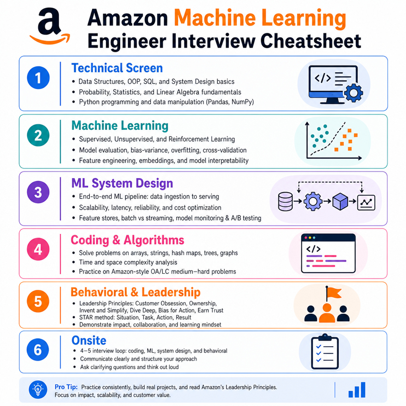
Technical Screen

Machine Learning

• Transformer Architectures And Attention — covered in depth under Onsite below.

• LLM Architecture, Tuning, And Evaluation — covered in depth under Onsite below.

• Logistic Regression And Linear Models — covered in depth under Onsite below.

• Evaluation, Statistical Inference, And Class Imbalance — covered in depth under Onsite below.

ML System Design

• Production ML Pipelines And System Design — covered in depth under Onsite below.

Coding & Algorithms

• Coding Algorithms And Data Structures — covered in depth under Onsite below.

• PyTorch Training And Model Implementation — covered in depth under Onsite below.

Behavioral & Leadership

• Leadership Principles, Ownership, And Measurable Impact — covered in depth under Onsite below.

Onsite

Machine Learning

What's being tested

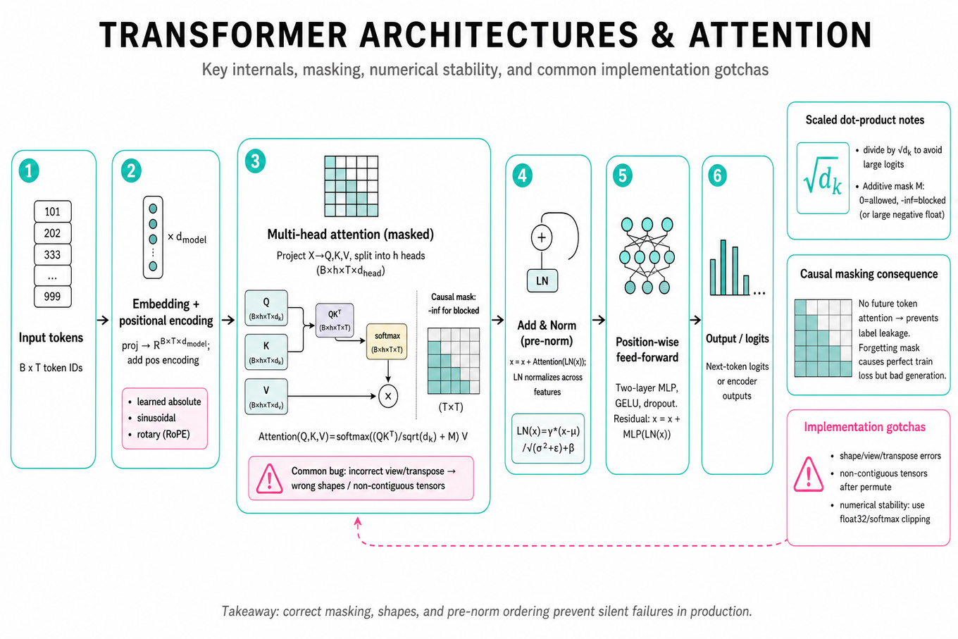
Interviewers are probing whether you understand Transformer internals well enough to implement, debug, train, and serve them—not just describe them at a high level. For a Machine Learning Engineer, the bar is shape reasoning, masking correctness, numerical stability, training efficiency, and knowing how architectural choices affect latency, memory, and model quality. Amazon cares because production ML systems often use Transformer-based encoders, decoders, rankers, retrieval models, and LLM-backed services where small implementation errors can silently degrade relevance, safety, or cost. Expect follow-ups that connect math to `PyTorch` tensors, GPU memory, distributed training, and online serving constraints.

Core knowledge

• Scaled dot-product attention computes $\mathrm{Attention}(Q,K,V)=\mathrm{softmax}\left(\frac{QK^\top}{\sqrt{d_k}} + M\right)V$ where $M$ is an additive mask, often 0 for allowed positions and -inf for blocked positions. The $\sqrt{d_k}$ scaling prevents large logits from saturating softmax.

• Multi-head attention projects an input $X \in \mathbb{R}^{B \times T \times d_{\text{model}}}$ into $Q,K,V$ tensors shaped roughly $B \times h \times T \times d_{\text{head}}$. Heads let the model learn different relation patterns; implementation bugs usually come from incorrect view, transpose, or non-contiguous tensors.

• Causal masking is mandatory for decoder-only language models. Token $t$ can attend only to positions $\leq t$, usually via a lower-triangular mask of shape $T \times T$. Forgetting this causes label leakage: training loss looks excellent, but generation quality fails.

• Decoder-only GPT-style blocks typically contain masked self-attention, a position-wise feed-forward network, residual connections, and normalization. A common pre-norm block is x = x + attention(LN(x)), then x = x + MLP(LN(x)), which improves deep-network training stability versus post-norm.

• Layer normalization normalizes across the feature dimension for each token independently: $\mathrm{LN}(x)=\gamma \frac{x-\mu}{\sqrt{\sigma^2+\epsilon}}+\beta$ where $\mu,\sigma^2$ are computed over hidden features, and $\gamma,\beta$ are learned per-feature parameters. Unlike batch norm, it does not depend on batch statistics.

• Position information is required because self-attention alone is permutation-equivariant. Common choices include learned absolute embeddings, sinusoidal embeddings, rotary position embeddings (`RoPE`), and relative position bias. For long-context serving, extrapolation behavior and `KV cache` compatibility matter.

• Feed-forward networks in Transformers are usually two linear layers with an activation such as `GELU`, often expanding hidden size by about 4x: $d_{\text{model}} \rightarrow 4d_{\text{model}} \rightarrow d_{\text{model}}$. In LLMs, gated variants like `SwiGLU` improve quality but increase parameter and memory considerations.

• Training-time memory is dominated by activations, attention matrices, and optimizer states. Full attention is $O(T^2)$ in sequence length and $O(BT^2)$ for attention probabilities; for long sequences, consider flash attention, gradient checkpointing, mixed precision, sequence packing, or sparse/local attention.

• Inference-time bottlenecks differ from training. Autoregressive decoding is sequential over generated tokens, but `KV cache` avoids recomputing keys and values for previous tokens, changing per-step attention from recomputing full prefix projections to attending against cached state. Cache memory grows with layers, heads, context length, and batch size.

• Mixture-of-Experts replaces dense MLPs with multiple expert networks and a learned router, often top-1 or top-2 routing. It increases parameter count without activating all parameters per token, but introduces load-balancing losses, capacity factors, token dropping risk, and distributed communication such as `all-to-all`.

• Transformers versus CNNs is about inductive bias and scaling tradeoffs. CNNs encode locality and translation equivariance through shared kernels, making them sample-efficient for images; Transformers learn global interactions with weaker priors but scale well with data, compute, multimodal inputs, and variable-length sequences.

• Evaluation and deployment require more than perplexity. For production MLE work, track offline loss, task metrics like `AUC` or `NDCG`, calibration, latency `p50/p99`, GPU memory, throughput, drift, and online/offline parity. A lower loss model may be unacceptable if it doubles serving cost or violates latency SLOs.

Worked example

For “Implement decoder-only GPT-style transformer,” a strong candidate first clarifies the expected scope: “Should I implement a minimal `PyTorch` module with token embeddings, positional embeddings, masked multi-head self-attention, MLP blocks, and logits, or also include training and generation?” They state assumptions early: input token IDs have shape B x T, vocabulary size is V, embedding dimension is C, number of heads divides C, and the model returns logits shaped B x T x V. The answer should be organized around four pillars: embeddings and positions, Transformer block structure, attention tensor shapes and causal mask, and output projection/loss.

The implementation skeleton would include `nn.Embedding` for tokens, either learned positional embeddings or `RoPE`, a stack of blocks using pre-norm residuals, and a final `LayerNorm` plus linear language-model head. The candidate should explicitly explain that q, k, and v are projected from x, reshaped from B x T x C to B x n_heads x T x head_dim, then attention scores become B x n_heads x T x T. A specific tradeoff to flag is whether to use a simple registered triangular mask, which is clear and interview-friendly, or optimized kernels like torch.nn.functional.scaled_dot_product_attention / FlashAttention for production efficiency. They should call out common edge cases: T exceeding configured context length, incorrect mask broadcasting, missing dropout behavior between train and eval, and using .view() after transpose without .contiguous() or .reshape(). A good close is: “If I had more time, I’d add generation with `KV cache`, unit tests for shape and causal leakage, and a small overfit test to verify the implementation learns.”

A second angle

For “Explain Layer Normalization in Transformers,” the same concept shifts from architecture construction to training stability and numerical behavior. Instead of writing modules end to end, the candidate should derive the equation, identify the normalized dimension, and explain the roles of $\gamma$, $\beta$, and $\epsilon$. The key MLE insight is that LayerNorm behaves consistently across small or variable batch sizes, which is important for sequence models and inference workloads where batch composition changes. A strong answer also distinguishes pre-norm from post-norm: pre-norm improves gradient flow in deeper networks, while post-norm matches the original Transformer but can be harder to optimize at scale. The interviewer may then pivot to why incorrect normalization placement can cause divergence, slow convergence, or degraded perplexity even when tensor shapes are correct.

Common pitfalls

Pitfall: Treating attention as “the model looks at important tokens” without discussing masks, shapes, or scaling.

That answer is too abstract for an MLE interview. A better response names $Q,K,V$, gives the attention equation, describes the B x heads x T x T score tensor, and explains how masking prevents future-token leakage in decoder-only models.

Pitfall: Confusing LayerNorm with BatchNorm.

BatchNorm normalizes using batch-level statistics and behaves differently between training and inference, while LayerNorm normalizes per token across hidden features and uses the same computation at inference. This distinction matters for variable-length sequences, small batches, autoregressive decoding, and distributed training.

Pitfall: Over-indexing on model architecture while ignoring production constraints.

Saying “use a larger Transformer” is incomplete if you do not mention latency, memory, throughput, quantization, `KV cache`, or online metrics. For an Amazon MLE, a strong answer connects architecture choices to deployability: model size, sequence length, batching strategy, GPU utilization, and monitoring for quality regressions.

Connections

Interviewers may pivot from this topic into distributed training, including data parallelism, tensor parallelism, pipeline parallelism, and MoE `all-to-all` communication. They may also ask about model compression techniques such as quantization, distillation, pruning, and low-rank adaptation, or about evaluation for LLM-style systems, including perplexity, task accuracy, hallucination checks, and latency/cost tradeoffs.

Further reading

• Attention Is All You Need — the original Transformer paper defining scaled dot-product attention, multi-head attention, positional encoding, and encoder-decoder blocks.

• Language Models are Unsupervised Multitask Learners — GPT-2 paper; useful for understanding decoder-only language modeling at scale.

• Switch Transformers: Scaling to Trillion Parameter Models with Simple and Efficient Sparsity — practical introduction to sparse MoE routing, capacity, and scaling tradeoffs.

Practice questions

What's being tested

Interviewers are probing whether you can reason about LLM architecture, fine-tuning, serving, and evaluation as an ML Engineer, not just recite Transformer terminology. You need to connect model internals—attention, tokenization, loss, routing, decoding—to operational concerns like latency, cost, validation coverage, safety regressions, and offline/online parity. Amazon cares because LLM-backed systems must be reliable under scale: small evaluation gaps can create customer-facing hallucinations, safety failures, or costly inference inefficiencies. A strong answer shows you can move between model math, training/evaluation pipelines, and production deployment tradeoffs.

Core knowledge

• Transformer decoder architecture is the default foundation for generative LLMs: token embeddings plus positional information feed stacked blocks of masked self-attention, MLP layers, residual connections, and layer normalization. At inference, autoregressive decoding predicts $p(x_t \mid x_{<t})$ one token at a time.

• Self-attention computes $\text{Attention}(Q,K,V)=\text{softmax}\left({QK^\top \over \sqrt{d_k}}\right)V$ and has $O(n^2)$ time and memory in sequence length $n$. For long contexts, mention mitigations such as KV caching, sliding-window attention, grouped-query attention, FlashAttention, retrieval augmentation, or chunking.

• Tokenization usually uses subword tokenizers such as BPE, WordPiece, or SentencePiece. Tokenization affects latency, multilingual quality, prompt length, and evaluation comparability. Edge cases include rare identifiers, URLs, code, non-Latin scripts, and whitespace-sensitive formats like JSON or Python.

• Pretraining optimizes next-token prediction over broad corpora, while instruction tuning teaches task-following behavior from curated prompt-response pairs. RLHF or DPO then aligns outputs with preference data. For an MLE, the key is data pipeline quality, reproducible training jobs, checkpointing, evaluation gates, and deployment compatibility.

• Surprisal measures how unexpected a token is: $I(x)=-\log p(x).$ With $\log_2$, units are bits; with natural log, units are nats. Average surprisal is cross-entropy, and perplexity is $\exp(H)$ for nats or $2^H$ for bits.

• Perplexity is useful for language-model fit but insufficient for assistant quality. A model can have better perplexity and worse helpfulness, safety, factuality, or instruction adherence. Pair it with task-level metrics such as exact match, pass@k, factuality checks, toxicity classifiers, human preference win rate, and calibrated LLM-as-judge evaluations.

• Mixture-of-Experts models activate a subset of expert MLPs per token, often top-1 or top-2 routed. This increases parameter count without proportional FLOPs, but creates load-balancing, routing instability, and distributed communication challenges. Training often adds auxiliary load-balancing losses to avoid expert collapse.

• MoE serving is not “free sparsity.” Tokens routed to different experts require all-to-all communication across devices, and batching becomes harder because expert assignment is data-dependent. Good answers discuss throughput, p99 latency, capacity factors, dropped tokens, expert parallelism, and fallback behavior during overload.

• Fine-tuning choices include full fine-tuning, LoRA, QLoRA, prefix tuning, and prompt tuning. LoRA injects low-rank adapters into weight matrices, reducing trainable parameters substantially. It is attractive when you need cheaper experimentation, safer rollback, and multiple task-specific adapters sharing one base model.

• Evaluation systems should test multiple layers: numerical integrity, data contamination, prompt formatting, model behavior, safety, latency, cost, and regression against known failures. A production validation suite often combines fixed golden sets, adversarial prompts, synthetic tests, shadow traffic, canaries, and human review for high-risk categories.

• Generation settings change quality and reproducibility. Temperature, top-p, top-k, max tokens, repetition penalties, and stop sequences affect hallucination, diversity, latency, and determinism. For validation, use deterministic decoding where possible, store seeds/configs, and separately test stochastic behavior distributions.

• RAG systems shift quality risk from only model weights to retrieval, chunking, embeddings, ranking, prompt assembly, and citation grounding. MLE-relevant evaluation includes recall@k for retrieval, answer faithfulness, source attribution, latency budget split, index freshness, and online/offline feature or embedding parity.

Worked example

For “Design an LLM quality validation system”, start by framing scope in the first 30 seconds: “Are we validating a base model, a fine-tuned assistant, or an end-to-end RAG application? What are the launch gates—quality, safety, latency, cost, or all of them? Is this for offline release validation, online monitoring, or both?” Then declare assumptions: a customer-facing assistant, multiple model versions, automated CI-style checks before deployment, and post-launch drift monitoring.

Organize the answer into four pillars. First, define evaluation coverage: curated golden prompts, task-specific benchmarks, safety/adversarial sets, regression tests from prior incidents, and representative production-like prompts with privacy-safe sampling. Second, define metrics: exact match or rubric score for structured tasks, LLM-as-judge preference with calibration, hallucination or groundedness for RAG, toxicity/safety rates, refusal correctness, latency p50/p95/p99, tokens per second, and cost per 1K requests. Third, describe the system architecture: model registry, prompt/version registry, evaluation runner, deterministic inference harness, result store, dashboard, and automated deployment gates. Fourth, cover online validation: shadow tests, canary rollout, alerting on metric regressions, drift detection in prompt distribution, and rollback.

A specific tradeoff to flag is LLM-as-judge versus human evaluation. LLM judges scale and catch many semantic issues, but they can be biased, brittle to prompt wording, and poorly calibrated for safety-critical categories; human review should remain the source of truth for high-risk or ambiguous cases. Close by saying: “If I had more time, I’d add red-team dataset refresh, inter-rater agreement tracking, and slice-based reporting by locale, device, prompt length, and task type.”

A second angle

For “Explain Transformers and MoE in LLMs”, the same concept shifts from validation-system design to architecture and scaling mechanics. Instead of leading with dashboards and release gates, lead with the Transformer block: masked self-attention, feed-forward layers, residual paths, layer norm, and autoregressive decoding. Then introduce MoE as a sparse replacement for dense feed-forward computation, where a router sends each token to a small number of experts. The MLE angle is not just “MoE has more parameters”; it is how routing affects training stability, GPU utilization, distributed all-to-all communication, checkpoint layout, serving latency, and monitoring for expert imbalance. A strong answer explicitly contrasts dense models’ simpler serving path with MoE’s better parameter/FLOP scaling but higher systems complexity.

Common pitfalls

Pitfall: Treating perplexity as the only quality metric.

Perplexity measures average next-token likelihood, not whether the assistant follows instructions, tells the truth, refuses unsafe requests correctly, or produces useful task outputs. A better answer says perplexity is one offline signal, then layers on task-specific, safety, human preference, and production telemetry metrics.

Pitfall: Explaining architecture without operational consequences.

A tempting answer defines attention, MoE, and RLHF correctly but never mentions batching, KV cache memory, latency, cost, rollout gates, or monitoring. For an ML Engineer interview, tie every architectural choice to training pipeline complexity, inference behavior, validation coverage, or deployment risk.

Pitfall: Being vague about evaluation data.

Saying “I’d test on a benchmark and some human labels” is too shallow. Stronger answers describe golden sets, adversarial sets, regression suites, slice analysis, contamination checks, deterministic generation configs, and a clear pass/fail threshold before model promotion.

Connections

Interviewers may pivot from here into RAG evaluation, model serving optimization, feature and embedding drift monitoring, or fine-tuning pipeline design. Be ready to discuss SageMaker, model registries, canary deployments, GPU memory bottlenecks, approximate nearest neighbor retrieval, and how offline validation connects to online rollback criteria.

Further reading

• Attention Is All You Need — original Transformer paper; essential for attention, positional encoding, and encoder-decoder architecture.

• Switch Transformers: Scaling to Trillion Parameter Models with Simple and Efficient Sparsity — practical MoE scaling, routing, and load-balancing tradeoffs.

• Training language models to follow instructions with human feedback — foundational InstructGPT paper covering instruction tuning and RLHF evaluation.

Practice questions

What's being tested

Interviewers are probing whether you understand gradient-boosted decision trees beyond “call XGBoost.fit().” For an Amazon Machine Learning Engineer, the important skill is connecting the learning algorithm to scalable training behavior: split finding, parallelism, sparse data handling, memory layout, distributed execution, and production tradeoffs. You should be able to explain why XGBoost can train efficiently on large tabular datasets, when it bottlenecks, and how you would tune or deploy it in a real ML pipeline. Strong answers combine algorithmic understanding with systems awareness: CPU cache, feature sparsity, distributed workers, evaluation, and online/offline parity.

Core knowledge

• Gradient boosting trains an additive ensemble of weak learners, usually trees:
  $\hat{y}_i^{(t)} = \hat{y}_i^{(t-1)} + \eta f_t(x_i)$
  Each new tree fits the negative gradient of the loss, so training is sequential across boosting rounds but parallelizable within each round.

• Second-order optimization is a key XGBoost idea. For loss $l(y_i, \hat{y}_i)$, it uses gradients $g_i$ and Hessians $h_i$ to score splits:
  $Gain = \frac{1}{2}\left[\frac{G_L^2}{H_L+\lambda} + \frac{G_R^2}{H_R+\lambda} - \frac{G^2}{H+\lambda}\right] - \gamma$
  where $G=\sum g_i$, $H=\sum h_i$.

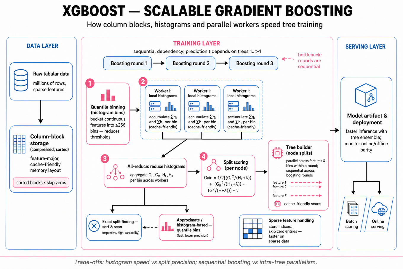
• Tree-level dependency limits parallelism: boosting rounds are inherently sequential because tree $t$ depends on predictions from trees $1..t-1$. The main parallelism is within a tree: evaluating candidate splits across features, data partitions, nodes, and histogram bins.

• Exact split finding sorts feature values and scans thresholds, which can be expensive for high-cardinality or large datasets. XGBoost supports approximate split finding and histogram-based algorithms, where continuous features are bucketed into quantile bins, reducing computation from many thresholds to typically 256 or fewer bins per feature.

• Histogram-based split finding accumulates gradient and Hessian statistics per feature bin. This is cache-friendly and enables parallel workers to build local histograms and reduce them. It trades some split precision for major speed and memory benefits, especially on datasets with millions of rows.

• Column block storage is central to XGBoost efficiency. Data is stored in compressed, sorted blocks by feature so that split scans access memory sequentially. This improves CPU cache locality and reduces random memory access, which often matters more than raw arithmetic throughput.

• Sparsity-aware split finding handles missing values and one-hot sparse features efficiently. For each split, XGBoost learns a default direction for missing values by evaluating whether missing entries should go left or right. Sparse-aware traversal avoids explicitly iterating over zeros in sparse matrices.

• Parallelism strategies include feature parallelism, data parallelism, node-level parallelism, and histogram parallelism. In practice, modern implementations often favor histogram/data parallelism because it maps well to multicore machines and distributed workers while minimizing synchronization overhead.

• Distributed training usually has each worker compute local gradient/Hessian histograms on a shard of data, then perform an AllReduce-style aggregation. Communication cost scales with number of features, bins, and active nodes, so wide datasets or deep trees can become network-bound.

• Regularization controls overfitting and serving cost. Important knobs include max_depth, min_child_weight, gamma, lambda, alpha, subsample, colsample_bytree, and learning_rate. Smaller trees and fewer boosting rounds improve latency and memory footprint for online inference.

• Evaluation discipline matters because boosted trees can overfit quickly. Use validation sets, early_stopping_rounds, calibration checks for probabilistic outputs, and task-appropriate metrics such as AUC, NDCG, logloss, RMSE, or MAPE. For ranking, use rank:pairwise, rank:ndcg, or rank:map objectives when appropriate.

• Production MLE concerns include feature consistency, model artifact size, inference latency, and drift monitoring. XGBoost models are often strong baselines for tabular prediction, but large ensembles can hurt p99 latency; you may need model compression, feature pruning, or a latency-aware hyperparameter search.

Worked example

For “Explain XGBoost Parallelism Strategies”, a strong candidate should first frame the answer around the constraint that boosting rounds are sequential, so the useful parallelism is mostly inside each tree. I would clarify whether the interviewer wants single-node multicore behavior, distributed training, or both, and I would state that I’m assuming histogram-based training on sparse tabular data. Then I’d organize the answer around four pillars: split finding, data representation, sparse handling, and distributed synchronization. For split finding, I’d explain that exact threshold search is expensive, while histogram-based methods aggregate $g_i$ and $h_i$ into bins and evaluate gains per bin. For systems behavior, I’d mention compressed column blocks, cache locality, and local histogram construction across threads.

Next, I’d describe distributed training: each worker processes a data shard, builds local histograms, and aggregates them so every worker can choose the same best split. The tradeoff I’d explicitly flag is that histogram binning reduces precision but dramatically lowers CPU, memory, and communication cost; for most large-scale tabular workloads this is the right tradeoff. I’d also discuss sparse-aware default directions for missing values because Amazon-scale datasets often have high-dimensional categorical or behavioral features with many zeros. I would close by saying that, if I had more time, I’d benchmark hist versus approx, tune max_bin, measure training throughput and validation quality, and check whether the bottleneck is CPU, memory bandwidth, or network communication.

A second angle

For “Explain key ML theory and techniques”, the same concept may appear as one component in a broader ML discussion rather than a standalone systems question. Here, you need a concise but accurate explanation that contrasts XGBoost with other model families such as neural networks, collaborative filtering models, or bandit algorithms. The framing should emphasize that XGBoost is a supervised, batch-trained, tree-ensemble method especially strong on structured tabular data. Instead of diving only into parallelism, connect the algorithm to training objective, regularization, missing-value handling, and deployment implications. The key is to show you can move between theory and practical MLE concerns without treating XGBoost as a black box.

Common pitfalls

Pitfall: Saying “XGBoost parallelizes trees” without qualification.

That answer is tempting but mostly wrong. Boosting rounds are sequential because each tree depends on residuals or gradients from the previous ensemble. A better answer is: “Trees are added sequentially, but split evaluation, histogram construction, feature scans, and distributed gradient aggregation can be parallelized within each boosting round.”

Pitfall: Explaining only model quality and ignoring systems tradeoffs.

For an MLE interview, “it has regularization and usually performs well on tabular data” is not enough. You should discuss training throughput, memory layout, sparse matrices, distributed communication, model size, and inference latency. Interviewers want to see that you can operate the model in a production pipeline, not just choose it in a notebook.

Pitfall: Treating histogram binning as a free optimization.

Histogram methods approximate continuous split points, so max_bin affects both accuracy and cost. Too few bins can underfit or miss important thresholds; too many bins increase memory and communication overhead. A strong answer names the tradeoff and proposes validation-based tuning rather than claiming one setting is universally best.

Connections

Interviewers may pivot from XGBoost to LightGBM, CatBoost, distributed training, feature stores, or model serving latency. They may also ask how boosted trees compare with deep learning for tabular data, how to monitor feature drift, or how to calibrate probability outputs before using scores in downstream ranking or decision systems.

Further reading

• XGBoost: A Scalable Tree Boosting System — the original paper explaining sparsity-aware split finding, weighted quantile sketch, cache-aware access, and distributed training.

• Elements of Statistical Learning, Chapter 10 — strong conceptual grounding for boosting, additive models, and tree ensembles.

• LightGBM: A Highly Efficient Gradient Boosting Decision Tree — useful contrast on histogram algorithms, leaf-wise growth, and large-scale GBDT optimization.

Practice questions

What's being tested

Interviewers are probing whether you understand linear models as trainable probabilistic systems, not just as `sklearn.linear_model.LogisticRegression` calls. For a Machine Learning Engineer, this matters because these models are still common in production ranking, ads, fraud, demand forecasting, and safety systems where latency, interpretability, calibration, and online/offline parity matter. Expect to derive losses and gradients, explain assumptions, choose regularization, diagnose failure modes like miscalibration or class imbalance, and connect model math to deployment behavior. A strong answer shows both mathematical fluency and production judgment: how the model is trained, evaluated, served, monitored, and fixed when data shifts.

Core knowledge

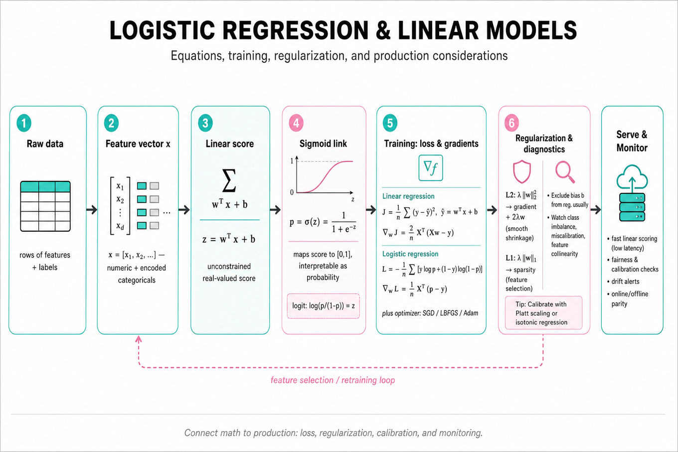
• Linear regression models a continuous target as $\hat{y}=w^\top x+b$ and usually minimizes mean squared error: $J(w,b)=\frac{1}{n}\sum_i(y_i-\hat{y}_i)^2.$ Its gradient is $\nabla_w J=\frac{2}{n}X^\top(Xw-y)$, which is the basis for batch, mini-batch, or stochastic gradient descent.

• Logistic regression models a Bernoulli probability using the sigmoid link: $p(y=1\mid x)=\sigma(z)=\frac{1}{1+e^{-z}},\quad z=w^\top x+b.$ The linear score is unconstrained, while the sigmoid maps it to $[0,1]$, making it suitable for binary classification and probability scoring.

• The logit link is $\log\frac{p}{1-p}=w^\top x+b$. This means each coefficient changes the log-odds additively; $e^{w_j}$ is the multiplicative odds ratio for a one-unit increase in feature $x_j$, assuming other features are fixed.

• Logistic regression is trained by maximizing the Bernoulli likelihood, equivalently minimizing binary cross-entropy: $L=-\frac{1}{n}\sum_i \left[y_i\log p_i+(1-y_i)\log(1-p_i)\right].$ The key gradient is simple: $\nabla_w L=\frac{1}{n}X^\top(p-y)$, often plus regularization terms.

• L2 regularization adds $\lambda\|w\|_2^2$ and shrinks coefficients smoothly, improving generalization under correlated or noisy features. L1 regularization adds $\lambda\|w\|_1$ and can produce sparse weights, useful for high-dimensional sparse features such as hashed categorical IDs.

• For logistic regression with L2, the gradient becomes $\nabla_w J=\frac{1}{n}X^\top(p-y)+2\lambda w,$ often excluding the bias term from regularization. Interviewers commonly check whether you regularize `b`; the usual answer is “no” unless there is a specific prior.

• Gradient descent choices matter operationally. Full-batch methods like L-BFGS are stable for smaller dense datasets; mini-batch SGD scales better for millions to billions of examples and sparse features. In production training pipelines, learning-rate schedules, shuffling, feature scaling, and checkpointing often matter more than the exact optimizer name.

• Feature scaling is critical for gradient-based training. Without standardization or normalization, large-scale features dominate updates, convergence slows, and regularization penalizes coefficients unevenly. Sparse binary/categorical features may not need standardization, but dense numerical features usually should.

• Calibration means predicted probabilities match empirical frequencies: among examples scored near $0.8$, roughly 80% should be positive. Logistic regression is often well-calibrated under correct specification, but imbalance, regularization, sampling bias, or distribution shift can require Platt scaling, isotonic regression, or post-training calibration on a holdout set.

• Evaluation metrics depend on serving use case. `ROC-AUC` measures ranking over thresholds and can look strong under class imbalance; `PR-AUC` is more informative when positives are rare. `LogLoss` evaluates probability quality, while calibration curves and expected calibration error catch probability miscalibration missed by AUC.

• Class imbalance can be handled with class weights, downsampling, threshold tuning, or loss reweighting, but each changes interpretation. If you train on sampled negatives, raw model probabilities may be biased; you may need prior correction or calibration against the true production distribution.

• Production failure modes include feature drift, label delay, training-serving skew, exploding logits from unbounded numerical inputs, and silent changes in feature distributions. MLEs should monitor `LogLoss`, `AUC`, calibration, prediction distribution, feature null rates, and online business guardrail metrics without owning raw ingestion infrastructure.

Worked example

For Explain Logistic Regression Fundamentals, a strong candidate starts by clarifying the setting: “Are we discussing binary classification, calibrated probability estimation, or thresholded decisions?” Then they state assumptions: labels are Bernoulli, features are fixed inputs, and the model uses a linear log-odds function passed through a sigmoid. The answer should be organized around four pillars: the probabilistic model, the loss derived from maximum likelihood, the optimization gradient, and practical evaluation/calibration.

The candidate would write $p_i=\sigma(w^\top x_i+b)$ and derive cross-entropy from the Bernoulli likelihood rather than presenting it as a memorized loss. They should mention the gradient $\nabla_w L=X^\top(p-y)/n$, because it explains why the update pushes probabilities down for false positives and up for false negatives. Next, they should discuss regularization: L2 for stability and lower variance, L1 for sparsity, and the bias term usually excluded. A concrete tradeoff to flag is that optimizing `LogLoss` improves probability quality, while selecting a threshold for precision/recall is a separate deployment decision. They can close by saying: “If I had more time, I’d validate calibration on a holdout set, compare `ROC-AUC` and `PR-AUC`, and check for training-serving skew or drift before deployment.”

A second angle

For Implement SGD for linear regression and derive gradients, the same foundation shifts from probabilistic classification to continuous regression and optimization mechanics. The candidate should derive MSE gradients, then show how mini-batch updates approximate the full gradient: $w \leftarrow w-\eta\nabla_w J_B$. The interviewer is less focused on sigmoid/log-odds and more on whether the candidate understands update loops, batch size, convergence, learning-rate sensitivity, and vectorized implementation. The production angle is similar: feature scaling, validation loss monitoring, checkpointing, and reproducibility are essential whether the model is linear or logistic. A good answer also notes numerical stability and stopping criteria rather than only writing the formula.

Common pitfalls

Pitfall: Treating logistic regression as “linear regression plus sigmoid.”

That answer is tempting but incomplete. What lands better is explaining that the sigmoid comes from modeling the log-odds linearly and fitting via Bernoulli maximum likelihood, which yields cross-entropy rather than MSE as the natural objective.

Pitfall: Confusing ranking quality with probability quality.

Saying “the model has high `ROC-AUC`, so probabilities are good” is analytically wrong. `ROC-AUC` can be high while calibration is poor; for probability-serving systems, mention `LogLoss`, calibration curves, `ECE`, and post-hoc calibration methods.

Pitfall: Giving only math and ignoring deployment constraints.

A derivation-only answer can sound academic for an MLE loop. Add production checks: feature scaling, sparse feature handling, train/serve parity, label leakage, drift monitoring, latency constraints, and whether thresholds or calibration are recomputed after retraining.

Connections

Interviewers may pivot from here to bias-variance tradeoff, regularization paths, online learning, feature engineering, or ranking metrics such as `NDCG`, `ROC-AUC`, and `PR-AUC`. They may also compare linear models with `XGBoost`, random forests, or neural networks, asking when the simpler model is preferable for interpretability, speed, or calibration.

Further reading

• The Elements of Statistical Learning — strong treatment of linear models, logistic regression, regularization, and model evaluation.

• [Pattern Recognition and Machine Learning, Bishop] — clear probabilistic view of generalized linear models and maximum likelihood.

• Probabilistic Machine Learning, Murphy — modern reference for probabilistic modeling, optimization, and calibration concepts.

Practice questions

What's being tested

Interviewers are probing whether you can evaluate ML systems under uncertainty, especially when labels are skewed, metrics disagree, or offline results may not transfer online. For an Amazon Machine Learning Engineer, this matters because deployed models often operate on rare but high-impact events: fraud, abuse, churn, defects, delayed deliveries, unsafe content, or low-frequency conversions. You need to reason about class imbalance, bias–variance, statistical significance, metric selection, and distributional differences without hiding behind a single accuracy number. Strong answers show that you can connect modeling choices to reliable evaluation, monitoring, and deployment decisions.

Core knowledge

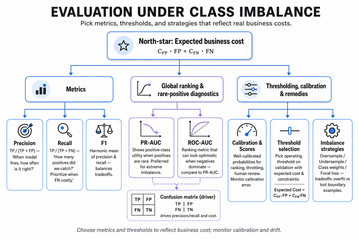
• Accuracy is usually misleading under class imbalance. If positives are 0.1%, a model that always predicts negative gets 99.9% accuracy but zero business or safety value. Prefer precision, recall, F1, PR-AUC, ROC-AUC, calibration error, and cost-weighted metrics.

• Confusion-matrix metrics encode different failure costs. precision = TP / (TP + FP) answers “when the model fires, how often is it right?” while recall = TP / (TP + FN) answers “how many true positives did we catch?” Fraud, abuse, and safety systems often prioritize recall subject to an acceptable false-positive budget.

• ROC-AUC can look good on heavily imbalanced data while PR-AUC reveals poor positive-class utility. ROC-AUC measures ranking across positives and negatives, but false positives can be cheap in the denominator when negatives dominate. PR-AUC is often more informative when positives are rare.

• Threshold selection is a deployment decision, not just a training artifact. A probabilistic model outputs scores; the operating threshold should be chosen using validation data, target constraints, and expected cost:
  $\text{Expected Cost} = C_{FP} \cdot FP + C_{FN} \cdot FN$
  Monitor whether the selected threshold remains valid after drift.

• Class imbalance strategies have tradeoffs. Oversampling positives can improve minority recall but increases overfitting risk; undersampling negatives reduces compute but may discard useful boundary examples; class-weighted loss changes optimization emphasis; focal loss downweights easy examples and is common in dense detection or extreme imbalance.

• Calibration matters when scores drive ranking, throttling, or human review queues. A model with good AUC can still produce poorly calibrated probabilities. Use Platt scaling, isotonic regression, Brier score, reliability diagrams, and expected calibration error when downstream systems interpret scores as probabilities.

• Bias–variance tradeoff explains underfitting and overfitting diagnostics. High bias appears as poor training and validation performance; high variance appears as strong training performance but weak validation performance. Remedies include more expressive models, regularization, feature improvements, early stopping, data augmentation, ensembling, or more representative data.

• Statistical inference is about uncertainty, not just point estimates. A p-value is $P(\text{data as or more extreme} \mid H_0)$, not the probability the null is true. For model comparisons, report confidence intervals via bootstrap, paired tests, or repeated folds rather than relying on tiny metric deltas.

• Paired evaluation is stronger than unpaired evaluation for model comparisons. If two models score the same examples, compare per-example losses or outcomes using a paired bootstrap, McNemar’s test for classification disagreements, or approximate randomization. This reduces variance versus comparing aggregate metrics from unrelated samples.

• Offline validation must reflect serving-time reality. Use time-based splits for nonstationary systems, entity-level splits to avoid user/item leakage, and shadow or canary deployments before full rollout. Leakage from future features, duplicate examples, or label-generation artifacts can create inflated offline metrics that fail in production.

• Population-difference testing depends on the object being compared. For a scalar feature, use t-test, Mann–Whitney U, or Kolmogorov–Smirnov depending on assumptions; for categorical distributions, use chi-square or Fisher’s exact test; for multivariate shift, use classifier-based two-sample tests, MMD, or energy distance.

• Architecture choices affect evaluation failure modes. CNNs encode locality and translation equivariance, often data-efficient for images; Transformers model long-range dependencies via attention but need more data and compute. In interviews, tie architecture back to inductive bias, data size, latency, and generalization—not just popularity.

Worked example

For “Explain imbalance, metrics, bias-variance, Transformers vs. CNNs”, a strong candidate would start by clarifying the task: “Is this binary classification, how rare is the positive class, what are the costs of false positives versus false negatives, and will the model be used for ranking, alerting, or automated action?” Then they would state an assumption, for example: “I’ll assume positives are rare, labels are reasonably reliable, and we can tune a threshold after training.” The answer can be organized into four pillars: evaluation metrics, imbalance handling, generalization diagnostics, and architecture tradeoffs.

For metrics, they should say that accuracy is insufficient and propose PR-AUC, precision at a fixed recall, recall at a fixed false-positive rate, and calibration if scores are consumed downstream. For imbalance handling, they should compare class-weighted loss, resampling, focal loss, and threshold tuning, while noting that resampling changes the training distribution and can affect calibration. For bias–variance, they should describe how training/validation curves diagnose underfitting versus overfitting and connect remedies to the observed pattern. For CNNs versus Transformers, they should avoid a generic “Transformers are better” claim and instead discuss inductive bias, data volume, compute, latency, and input modality.

One explicit tradeoff to flag: maximizing recall can overwhelm a human review queue or downstream service with false positives, so the threshold should often be selected under an operational constraint such as “95% recall with precision above 20%” or “no more than 10,000 alerts per day.” A strong close would be: “If I had more time, I’d validate the selected metric with a cost model, check calibration, run a paired significance test against the baseline, and monitor class prior drift after deployment.”

A second angle

For “Test whether two user populations differ”, the same evaluation mindset shifts from model quality to distributional comparison. A strong answer first asks what “differ” means: label rate, feature distribution, prediction-score distribution, calibration, or downstream error rate. If the goal is to compare one scalar metric, a confidence interval or hypothesis test may suffice; if the goal is broad covariate shift detection, a classifier-based two-sample test can reveal whether one population is predictable from features. The MLE framing should connect the test to model risk: if two populations differ materially, the model may require segmented evaluation, recalibration, reweighting, or separate thresholds. The constraint is that statistical significance at huge sample sizes may detect trivial differences, so effect size and operational impact must be reported alongside p-values.

Common pitfalls

Pitfall: Saying “use F1 for imbalanced data” as a universal answer.

F1 assumes precision and recall are equally important, which is often false. A better answer explains the cost of each error type, chooses metrics such as precision at fixed recall or recall at fixed false-positive rate, and justifies the operating threshold.

Pitfall: Treating p-values as proof that one model is better.

A small p-value does not imply a meaningful effect size, and repeated metric checks can inflate false positives. Strong candidates mention confidence intervals, paired comparisons, multiple-testing correction when relevant, and whether the metric delta is large enough to matter operationally.

Pitfall: Explaining bias–variance only as textbook definitions.

Interviewers expect diagnostic reasoning: what do training and validation curves look like, what interventions follow, and how would you verify improvement? Tie high variance to regularization, more data, early stopping, or simpler models; tie high bias to better features, higher-capacity models, or reduced regularization.

Connections

Interviewers may pivot from here into model monitoring, especially drift detection, online/offline metric parity, and alerting on calibration or class-prior shifts. They may also connect to A/B testing, causal inference, ranking evaluation, or model serving constraints such as latency-driven thresholding and fallback behavior.

Further reading

• “The Relationship Between Precision-Recall and ROC Curves” by Davis and Goadrich — canonical paper explaining why PR curves are often preferable under class imbalance.

• “Imbalanced Learning: Foundations, Algorithms, and Applications” by He and Ma — deep treatment of resampling, cost-sensitive learning, and evaluation under skewed labels.

• “The Elements of Statistical Learning” by Hastie, Tibshirani, and Friedman — strong reference for bias–variance, model selection, regularization, and supervised learning evaluation.

Practice questions

What's being tested

Interviewers are probing whether you can explain personalized recommendation methods at both the modeling and production levels: how collaborative filtering learns user–item affinity, how bandits allocate traffic under uncertainty, and how these methods are evaluated and served safely. For an Amazon Machine Learning Engineer, this matters because recommendations, ads, search ranking, merchandising, and content placement all require scalable personalization under latency, freshness, cold-start, and feedback-loop constraints. You should be able to compare algorithms, state modeling assumptions, discuss offline versus online evaluation, and identify deployment risks like exploration bias, popularity bias, and training-serving skew.

Core knowledge

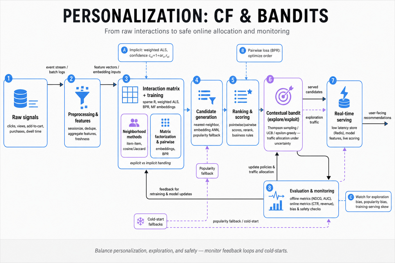
• Collaborative filtering assumes users with similar historical behavior will prefer similar items. The core signal is a sparse user–item interaction matrix $R \in \mathbb{R}^{m \times n}$, where entries may represent ratings, purchases, clicks, views, dwell time, or add-to-cart events.

• Neighborhood-based methods compute similarity between users or items, then recommend based on nearest neighbors. Item-item collaborative filtering is often more stable than user-user filtering because item relationships change more slowly; similarity can use cosine, Jaccard, Pearson correlation, or adjusted cosine.

• Matrix factorization represents each user and item with latent vectors:
  $\hat r_{ui} = p_u^\top q_i + b_u + b_i + \mu$
  where $p_u$ and $q_i$ are embeddings, $b_u$ and $b_i$ are biases, and $\mu$ is the global mean. This scales better than neighborhood methods for large sparse matrices.

• Explicit feedback uses ratings or thumbs-up signals and often optimizes squared error, but ratings are sparse and biased toward highly engaged users. Implicit feedback uses clicks, purchases, views, or streams; missing entries are not true negatives, so methods like weighted ALS use confidence $c_{ui}=1+\alpha r_{ui}$.

• Pointwise losses predict an absolute label such as click probability or rating. Pairwise losses, such as Bayesian Personalized Ranking (BPR), optimize relative ordering: a user should rank an observed item above an unobserved one, often with loss $-\log \sigma(\hat r_{ui} - \hat r_{uj})$.

• Cold start is a central production issue. New users need contextual, demographic, query, session, or popularity-based fallbacks; new items need content features, catalog metadata, image/text embeddings, or exploration traffic before collaborative signals accumulate.

• Approximate nearest neighbor retrieval is common for candidate generation from learned embeddings. Systems often use `FAISS`, `ScaNN`, or `Annoy` to retrieve top-K candidates under millisecond-level latency, then send them to a heavier ranker.

• Bandit algorithms address the exploration–exploitation tradeoff: exploiting known high-performing actions maximizes short-term reward, while exploring uncertain actions improves future decisions. Regret is commonly defined as $R_T = T\mu^\* - \sum_{t=1}^{T} r_t$.

• Epsilon-greedy chooses the current best arm with probability $1-\epsilon$ and explores randomly with probability $\epsilon$. It is simple and production-friendly, but uniform exploration can waste traffic on clearly poor arms unless $\epsilon$ decays or arms are filtered.

• Upper Confidence Bound (UCB) chooses actions using optimism under uncertainty, for example:
  $a_t = \arg\max_a \left(\hat\mu_a + c\sqrt{\frac{\log t}{N_a}}\right)$
  It naturally explores under-sampled arms, but assumes reward estimates and confidence terms are meaningful and comparable.

• Thompson sampling samples from each arm’s posterior distribution and chooses the arm with the highest sampled reward. For Bernoulli rewards, a common model is `Beta(alpha, beta)` per arm; it often performs well in practice and handles uncertainty more smoothly than deterministic UCB.

• Contextual bandits condition action choice on features such as user, item, query, device, time, and session context. Production implementations may use linear models, gradient-boosted trees, or neural rankers, but must log propensities to support unbiased offline evaluation via inverse propensity scoring.

Worked example

For Explain Collaborative Filtering Approaches, a strong candidate should first frame the problem: “Are we recommending products, videos, or ads; do we have explicit ratings or implicit events; and is the goal candidate generation, ranking, or both?” Then declare assumptions: “I’ll assume a large sparse user–item matrix with implicit feedback such as clicks and purchases, and a latency-sensitive serving path.” A clean answer has four pillars: neighborhood methods, matrix factorization, implicit-feedback modeling, and production considerations.

Start with neighborhood methods because they are intuitive: user-user similarity recommends what similar users liked, while item-item similarity recommends items co-consumed with items the user interacted with. Then move to matrix factorization: learn user and item embeddings using ALS, SGD, or BPR, and score with a dot product. For implicit feedback, emphasize that unobserved does not mean disliked; weighted ALS or sampled negatives are better than treating every missing cell as a zero.

The tradeoff to flag explicitly is interpretability and simplicity versus scalability and representation power. Item-item models are easy to debug and cache, while factorization models handle sparsity better and produce embeddings usable in `FAISS`-style retrieval. Close by saying: “If I had more time, I would discuss cold start using content features, offline metrics like `Recall@K` and `NDCG@K`, and online validation with guardrail metrics such as latency and engagement quality.”

A second angle

For Explain Multi-Armed Bandit Principles, the framing shifts from learning static preferences to making sequential decisions while collecting data. Instead of asking “Which items are most similar?” the interviewer wants to hear “How do we allocate impressions among uncertain choices while minimizing regret?” The same personalization setting applies, but bandits are especially relevant when launching new recommendations, exploring new items, or selecting among ranking policies. A strong answer compares epsilon-greedy, UCB, and Thompson sampling, then extends to contextual bandits where user and item features affect the best action. The key production constraint is that exploration changes the data distribution, so the system must log chosen actions, rewards, and action probabilities for evaluation and retraining.

Common pitfalls

Pitfall: Treating missing interactions as negative labels.

In recommender systems, most user–item pairs are unobserved because the user never saw the item, not because they disliked it. A better answer distinguishes exposure, click, purchase, and rating signals, then explains confidence-weighted implicit feedback or negative sampling.

Pitfall: Describing bandits as “just A/B testing with automation.”

A/B tests estimate average treatment effects under fixed allocation, while bandits adapt allocation over time based on observed rewards. For an MLE role, mention regret, logging propensities, delayed rewards, non-stationarity, and guardrails before claiming a bandit is production-ready.

Pitfall: Staying at textbook algorithm names without deployment details.

Saying “use matrix factorization” or “use Thompson sampling” is not enough. Interviewers expect you to connect the algorithm to feature freshness, offline/online parity, candidate retrieval latency, drift monitoring, cold-start fallbacks, and safe rollout through shadow mode, canaries, or limited traffic.

Connections

Interviewers may pivot from this topic into learning-to-rank, embedding retrieval, offline recommender evaluation, feature stores, model calibration, or online experimentation. Be ready to explain how candidate generation and ranking interact, how `Recall@K` differs from `NDCG@K`, and why offline gains may fail to translate online due to feedback loops or exposure bias.

Further reading

• Matrix Factorization Techniques for Recommender Systems — Koren, Bell, Volinsky — classic overview of latent factor models for collaborative filtering.

• Collaborative Filtering for Implicit Feedback Datasets — Hu, Koren, Volinsky — foundational paper for weighted implicit-feedback matrix factorization.

• A Contextual-Bandit Approach to Personalized News Article Recommendation — Li et al. — practical introduction to contextual bandits, exploration, and offline policy evaluation.

Practice questions

ML System Design

What's being tested

Interviewers are probing whether you can reason about distributed training as an end-to-end ML engineering problem: how model computation, memory, communication, and convergence interact when scaling beyond one accelerator or one host. You should be able to explain data parallelism, tensor/model parallelism, pipeline parallelism, expert parallelism, and the collective communication primitives that make them work. Amazon cares because large-scale training systems directly affect GPU utilization, cost per experiment, training reliability, and iteration speed for production ML systems. A strong answer connects algorithms to systems metrics: throughput, memory footprint, communication volume, straggler sensitivity, and model quality.

Core knowledge

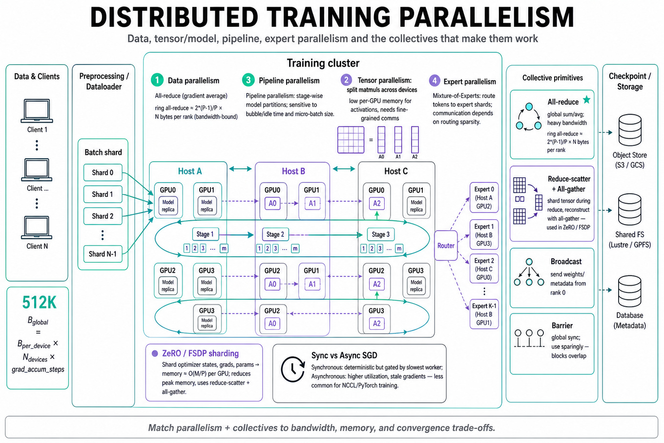
• Data parallelism replicates the model on each worker, shards the batch, computes local gradients, then synchronizes gradients with all-reduce. Effective global batch size is $B_\text{global}=B_\text{per device}\times N_\text{devices}\times \text{grad accumulation steps}$, which can require learning-rate scaling and warmup.

• Synchronous SGD gives deterministic step boundaries and simpler convergence reasoning, but the slowest worker gates every iteration. Asynchronous training can improve hardware utilization but introduces stale gradients; it is less common for large PyTorch/NCCL deep learning training where convergence stability matters.

• All-reduce combines values across ranks and returns the result to every rank, commonly used for gradient averaging. Ring all-reduce moves roughly $2\frac{P-1}{P}N$ bytes per rank for $P$ workers and tensor size $N$, making bandwidth the dominant bottleneck for large gradients.

• Reduce-scatter partitions a reduced tensor across ranks, while all-gather reconstructs the full tensor from shards. DeepSpeed ZeRO and PyTorch FSDP exploit this: shard optimizer states, gradients, and parameters to reduce memory from roughly $O(M)$ per GPU toward $O(M/P)$ for model state size $M$.

• Broadcast sends data from one rank to all others, often used to initialize model weights or distribute metadata. Barrier synchronizes ranks but should be used sparingly; unnecessary barriers can hide performance bugs and reduce overlap between compute and communication.

• Tensor parallelism splits individual matrix operations across devices, common in Transformer MLP and attention projections. It reduces per-device memory and compute, but introduces collectives such as all-reduce or all-gather inside every layer, so it is sensitive to fast intra-node links like NVLink.

• Pipeline parallelism partitions layers across devices and sends activations forward and gradients backward. It improves model-size scalability but creates pipeline bubbles; schedules like 1F1B reduce idle time, while microbatch count controls the tradeoff between utilization and activation memory.

• Expert parallelism in Mixture-of-Experts models routes tokens to different expert networks. It usually requires all-to-all communication: tokens are exchanged by expert assignment, processed locally, then returned. Load imbalance is a core issue, so routing capacity factors and auxiliary load-balancing losses matter.

• Hybrid parallelism combines data, tensor, pipeline, and expert parallelism. A practical design maps high-traffic collectives to fastest links: tensor parallel inside a node, pipeline across nodes, and data parallel across replicas. Poor placement can make the network, not the GPU, the training bottleneck.

• Gradient accumulation simulates larger batches without synchronizing every microbatch. In PyTorch DistributedDataParallel, no_sync() avoids intermediate all-reduces, reducing communication frequency, but increases optimizer-step latency and may affect convergence if the effective batch becomes too large.

• XGBoost parallelism differs from neural training: histogram-based split finding builds feature histograms over row shards, then merges histograms across workers. Sparse-aware split finding skips missing entries and uses default directions; performance depends on cache-friendly column blocks, quantile sketching, and communication of compact histograms rather than dense gradients.

• Performance debugging should separate compute, memory, and communication. Track GPU utilization, step time, tokens/sec or samples/sec, network throughput, collective time, and variance across ranks. Tools include NVIDIA Nsight Systems, PyTorch Profiler, NCCL_DEBUG, DeepSpeed logs, and rank-level timing.

Worked example

For Explain parallelism and collectives in training, a strong candidate would start by clarifying the target setting: “Are we training a Transformer-like dense model, how many GPUs and nodes are available, and is the limiting factor memory, throughput, or time-to-convergence?” Then they would declare assumptions, such as using PyTorch, NCCL, homogeneous GPUs, and synchronous training.

The answer skeleton should have four pillars: first, describe data parallelism as the default scaling strategy and explain gradient all-reduce; second, introduce model/tensor parallelism when the model or activations do not fit on one GPU; third, discuss pipeline parallelism for very deep models and the bubble/utilization tradeoff; fourth, name core collectives and map them to training operations. The candidate should explicitly call out that collectives are not interchangeable: all-reduce is natural for replicated-gradient averaging, all-gather/reduce-scatter are natural for sharded parameters and optimizer states, and all-to-all is central for MoE token routing.

A concrete tradeoff to flag is memory versus communication. FSDP or ZeRO-3 can enable larger models by sharding parameters, gradients, and optimizer state, but may increase all-gather frequency around layer execution; this can hurt throughput if network bandwidth is weak. The candidate should also mention overlapping communication with backpropagation using gradient buckets, because practical training performance depends on hiding all-reduce latency behind compute.

A good close would be: “If I had more time, I’d propose a parallelism layout based on model size and cluster topology, then validate it with per-rank profiling: step time breakdown, collective duration, GPU utilization, and scaling efficiency.”

A second angle

For Explain Transformers and MoE in LLMs, the same distributed-systems concepts appear, but the framing shifts from generic training to architecture-specific scaling. Dense Transformer layers often use tensor parallelism for attention and MLP projections, where all-reduce or all-gather appears inside each block. MoE adds expert parallelism: tokens are dynamically routed to experts, which makes all-to-all communication and load balancing first-class design constraints. The key difference is that MoE increases parameter count without activating every parameter for every token, so the MLE must reason about capacity factor, dropped tokens, expert imbalance, and communication overhead rather than only gradient synchronization.

Common pitfalls

Pitfall: Treating “distributed training” as just data parallel all-reduce.

That answer is incomplete for modern large models. Data parallelism is the simplest baseline, but the interviewer expects you to know when memory forces sharding, tensor parallelism, pipeline parallelism, or hybrid layouts. A better answer starts with data parallelism, then explains the failure modes that motivate other strategies.

Pitfall: Naming collectives without explaining what data moves.

Saying “use NCCL all-reduce” is not enough. You should identify whether the tensor being moved is gradients, parameters, activations, token embeddings, histograms, or optimizer state. This distinction shows you understand both correctness and performance.

Pitfall: Ignoring convergence and ML quality when optimizing systems throughput.

A tempting but weak answer maximizes samples/sec by increasing global batch size indefinitely. A stronger MLE answer notes that larger batches can require learning-rate scaling, warmup, gradient clipping, and validation monitoring; throughput gains are only useful if time-to-quality improves.

Connections

Interviewers may pivot from this topic into training pipeline design, model checkpointing, fault tolerance, GPU memory optimization, or serving-time model parallelism. They may also connect it to feature engineering and distributed tree training through XGBoost, where the same communication-versus-computation tradeoff appears but with histograms and split statistics instead of neural gradients.

Further reading

• “Megatron-LM: Training Multi-Billion Parameter Language Models Using Model Parallelism” — foundational paper on tensor and pipeline parallelism for large Transformer training.

• “ZeRO: Memory Optimizations Toward Training Trillion Parameter Models” — explains optimizer, gradient, and parameter sharding tradeoffs used by DeepSpeed.

• “XGBoost: A Scalable Tree Boosting System” — covers histogram/quantile-based tree training, sparsity handling, and systems optimizations behind distributed XGBoost.

Practice questions

What's being tested

Interviewers are probing whether you can design a production ML system that is trainable, deployable, measurable, and maintainable after launch. For a Machine Learning Engineer at Amazon, this means translating a model idea into a reliable pipeline: data contracts, feature computation, training, evaluation, deployment, monitoring, rollback, and retraining. The focus is not just “which model would you use,” but how you prevent offline/online skew, detect regressions, control latency and cost, and prove the model improves customer-facing outcomes. Strong answers show ownership of ML-specific infrastructure without drifting into raw storage, message-broker, or product-strategy design.

Core knowledge

• Problem framing comes before architecture: define prediction target, inference mode, latency budget, freshness requirement, retraining cadence, failure tolerance, and evaluation metric. A fraud model, recommender, and LLM validator can all use pipelines, but their label delay, calibration needs, and serving constraints differ sharply.

• Training pipelines should be reproducible: version the dataset snapshot, feature code, labels, model code, hyperparameters, container image, and random seed. In practice, this means using systems like SageMaker Pipelines, Kubeflow Pipelines, MLflow, or Airflow for orchestration and lineage.

• Feature engineering must address offline/online parity. If training uses batch-computed aggregates but serving recomputes them differently, you get training-serving skew. A feature store such as SageMaker Feature Store, Feast, or Tecton helps by sharing transformation definitions and maintaining online/offline views.

• Label design is often the hardest part. Define observation windows, prediction windows, censoring rules, and leakage boundaries. For example, if predicting conversion within 7 days, features must be computed strictly before exposure time $t$, and labels should be $y=\mathbb{1}[\text{conversion in }(t,t+7d]]$.

• Model evaluation should combine discrimination, calibration, ranking, and slice metrics. Use AUC-ROC, PR-AUC, NDCG@K, MAP@K, log loss, or Brier score depending on the task. Calibration can be checked with expected calibration error: $ECE=\sum_b \frac{|B_b|}{n}|\text{acc}(B_b)-\text{conf}(B_b)|$.

• Validation gates prevent bad models from deploying. Gates usually include schema checks, feature distribution checks, label leakage tests, offline metric thresholds, regression tests against a baseline, fairness/safety slices, latency benchmarks, and canary results. A model should fail closed if core validation data is missing.

• Deployment patterns include batch scoring, synchronous real-time inference, asynchronous inference, shadow deployment, canary rollout, blue/green deployment, and A/B testing. For high-QPS services, latency targets should include p50, p95, and p99, not just average latency.

• Serving architecture depends on model size and freshness. Tree models like XGBoost are often cheap to serve with millisecond latency; deep ranking models may need GPU or vector retrieval; LLM systems need prompt templates, retrieval context, safety filters, caching, token budgets, and fallback behavior.

• Monitoring must separate data drift, prediction drift, concept drift, and performance decay. Useful signals include feature null rate, embedding norm distribution, population stability index PSI, KL divergence, prediction score histograms, calibration by slice, latency, error rate, and business proxy metrics.

• Retraining strategy should match label delay and drift speed. Common choices are scheduled retraining, performance-triggered retraining, active-learning loops, or human-in-the-loop review. Avoid automatic promotion from retraining alone; require evaluation gates and staged deployment.

• LLM validation needs layered evaluation: prompt/unit tests, retrieval quality, factuality, toxicity, hallucination rate, jailbreak robustness, latency, cost per request, and human preference. Metrics can include exact match, semantic similarity, rubric-based judge scores, pairwise win rate, and safety violation rate.

• Scalability choices should be ML-driven, not infrastructure theater. Use pandas or DuckDB for small offline experiments, distributed Spark or Ray for hundreds of millions of rows, and approximate nearest neighbor indexes like FAISS, ScaNN, or HNSW when embedding retrieval exceeds brute-force feasibility.

Worked example

For Build an end-to-end ML pipeline, a strong candidate starts by clarifying: “What is the prediction target, how quickly do predictions need to be served, how delayed are labels, and what is the cost of false positives versus false negatives?” They would also state assumptions, such as “I’ll assume this is a supervised binary prediction problem with daily retraining, batch feature generation, and online low-latency inference.” The answer should be organized around four pillars: data and label definition, feature generation with offline/online parity, model training and evaluation, and deployment plus monitoring.

The candidate might describe a pipeline that validates input schemas, creates point-in-time-correct training examples, trains a baseline model such as XGBoost or a neural model depending on data shape, evaluates against offline metrics and business-aligned slices, then registers the model in a model registry. Deployment would use a canary or shadow stage before full rollout, with rollback to the previous model if p99 latency, error rate, or calibration exceeds thresholds. One explicit tradeoff to flag is batch versus real-time features: batch features are simpler and cheaper but may be stale; real-time features improve freshness but increase serving complexity and skew risk. A strong close would be: “If I had more time, I’d discuss retraining triggers, human review for ambiguous labels, and how I’d run an online experiment before making the model the default.”

A second angle

For Design an LLM quality validation system, the same production ML principles apply, but the artifacts and failure modes change. Instead of only validating numeric features and supervised labels, you validate prompts, retrieved context, generated text, safety filters, and model-version behavior across regression suites. Offline evaluation may combine curated golden sets, adversarial prompts, rubric-based human review, and LLM-as-judge scoring, while online monitoring tracks hallucination reports, refusal rate, latency, token cost, and safety violations. The key constraint is that LLM quality is multi-dimensional: a model can improve helpfulness while worsening factuality or policy compliance, so promotion needs multiple gates rather than a single aggregate score.

Common pitfalls

Pitfall: Optimizing only for a headline metric like AUC.

A tempting answer is “train a model, compare AUC, deploy if it improves.” That misses calibration, threshold selection, slice regressions, latency, and online impact. A stronger answer maps metrics to the decision being automated: ranking needs NDCG@K, probability decisions need calibration, and customer-impacting launches need staged online validation.

Pitfall: Starting with tools before requirements.

Saying “I’ll use SageMaker, Spark, Kafka, and Kubernetes” without clarifying target, label delay, freshness, and latency sounds shallow. Interviewers want the design to follow from constraints. Lead with the ML contract, then choose tools only where they solve a specific production problem.

Pitfall: Treating monitoring as dashboards only.

“Monitor drift” is not enough. Specify which distributions you monitor, what thresholds trigger alerts, who or what responds, and whether the response is rollback, retraining, feature disablement, or human review. Good monitoring connects symptoms to operational actions.

Connections

Interviewers often pivot from this topic into feature stores, model evaluation and calibration, online experimentation, LLM safety evaluation, or recommender/ranking system design. They may also ask about adjacent storage or serving systems, but for an MLE answer, keep the focus on ML artifacts, model lifecycle, and customer-safe deployment.

Further reading

• Hidden Technical Debt in Machine Learning Systems — classic paper on why production ML complexity comes from glue code, data dependencies, and monitoring gaps.

• Google: Rules of Machine Learning — practical guidance on metrics, launch stages, feature management, and iteration.

• Google Cloud: MLOps Continuous Delivery and Automation Pipelines in Machine Learning — useful reference architecture for pipeline maturity levels and automated validation gates.

Practice questions

Coding & Algorithms

What's being tested

Amazon MLE coding screens test whether you can turn ML-adjacent production tasks into clean algorithms: batching, clustering, training loops, graph reachability, interval allocation, and top-k retrieval. Interviewers look for correct data structures, complexity analysis, edge-case handling, and code that would survive inside a training or serving pipeline.

Patterns & templates

• K-means implementation — initialize centroids, assign by nearest distance, recompute means; stop on max iterations or centroid shift $\lt \epsilon$.

• Interval merging / allocation — sort by start time, scan once, merge or consume ranges; usually O(n log n) time from sorting.

• Top-k frequency retrieval — use collections.Counter plus heapq.nlargest for O(n log k), or bucket counts for bounded frequencies.

• Directed cycle check — adding edge u -> v creates a cycle iff u is reachable from v; solve with DFS/BFS.

• PyTorch training loop — order matters: model.train(), move tensors to device, optimizer.zero_grad(), forward, loss, backward(), step().

• Bucket batching optimization — sort or group examples by sequence length/cost, then pack batches to reduce padding and GPU underutilization.

• Event-driven queues — model backorders or pending work with deque, heapq, or ordered maps; define FIFO vs priority semantics explicitly.

Common pitfalls

Pitfall: Writing ML pseudocode without executable edge handling, such as empty clusters in K-means or zero-length batches in bucketing.

Pitfall: Missing complexity tradeoffs; Amazon interviewers expect O(V+E), O(n log n), memory cost, and when the approach breaks at scale.

Pitfall: In PyTorch loops, forgetting optimizer.zero_grad() or device movement silently produces wrong training behavior or runtime errors.

Practice these

The practice cards below cover the canonical variants — solve all of them and time yourself.

Practice questions

What's being tested

Tests implementation fluency for ML algorithms and `PyTorch` models: tensor shapes, gradients, optimization steps, and clean modular code. Interviewers look for whether you can translate math/model architecture into correct, runnable code while handling edge cases and complexity.

Patterns & templates

• PyTorch training loop — `model.train()`, move batch to `device`, `optimizer.zero_grad()`, `loss.backward()`, `optimizer.step()`; track loss without retaining graphs.

• Tensor shape discipline — state shapes at every layer, e.g. transformer input (B, T, C), attention logits (B, H, T, T); most bugs are silent broadcasting errors.

• Masked self-attention — compute QK^T / sqrt(d_k), apply causal mask with masked_fill(..., -inf), then softmax; ensure no future-token leakage.

• Residual block template — x = x + attention(norm(x)), then x = x + mlp(norm(x)); know pre-norm vs post-norm stability tradeoff.

• Manual SGD derivation — for MSE linear regression, $\nabla_w = \frac{2}{n}X^T(Xw-y)$ and $\nabla_b = \frac{2}{n}\sum(\hat y-y)$; update in-place carefully.

• K-means loop — assign points to nearest centroid, recompute means, stop on convergence or max iterations; handle empty clusters deterministically.

• Classic DSA helpers — interval merge via sort by start O(n log n); top-k frequency via heap O(n log k) or bucket sort O(n).

Common pitfalls

Pitfall: Forgetting `optimizer.zero_grad()` accumulates gradients across batches and produces misleadingly unstable training.

Pitfall: Building a GPT block without a causal mask turns it into bidirectional attention and invalidates decoder-only behavior.

Pitfall: Explaining algorithms conceptually but not giving tensor dimensions, update equations, or runtime complexity will look shallow.

Practice these

The practice cards below cover the canonical variants — solve all of them and time yourself.

Practice questions

Behavioral & Leadership

What's being tested

Interviewers are probing whether you can show end-to-end ownership of machine learning work: framing an ambiguous problem, making technical decisions, deploying safely, measuring impact, and taking responsibility when reality diverges from the plan. For an Amazon Machine Learning Engineer, this matters because models are not judged by offline scores alone; they must improve customer-facing or operational outcomes while meeting constraints on latency, cost, reliability, privacy, and maintainability. Strong answers connect Leadership Principles like Ownership, Dive Deep, Bias for Action, Are Right A Lot, and Insist on the Highest Standards to concrete MLE artifacts: training pipelines, feature quality, model evaluation, deployment strategy, monitoring, rollback plans, and measurable business or platform impact. The interviewer is listening for evidence that you did not just “build a model,” but owned the full production ML lifecycle and could quantify the result.

Core knowledge

• STAR with technical depth is the baseline: Situation, Task, Action, Result should include model context, constraints, and measurable outcome. For MLE interviews, “Result” should include metrics like AUC, NDCG@K, precision@recall, p95 latency, GPU-hours, inference cost/request, CTR, or defect rate.

• Ownership scope should cover the full ML path: data and label assumptions, feature generation, training pipeline, offline evaluation, serving path, deployment strategy, monitoring, and incident response. You do not need to own every upstream system, but you should show how you validated dependencies and mitigated risk.

• Measurable impact needs a before/after baseline. Cost reduction can be expressed as $\text{savings} = (\text{baseline unit cost} - \text{new unit cost}) \times \text{volume} - \text{migration cost}$ For example: reducing average inference cost from $0.42 to $0.19 per 1,000 predictions at 2B predictions/month yields about $460K/month before one-time costs.

• Offline/online metric alignment is a common MLE ownership topic. A better AUC or lower validation log_loss is not enough if the online metric, such as conversion_rate, latency, or manual-review load, regresses. Strong answers explain guardrail metrics and why the offline proxy was trusted or insufficient.

• Deployment safety shows mature ownership. Mention shadow testing, canary releases, A/B testing, feature flags, and rollback criteria. For high-risk models, describe staged rollout such as 1%, 5%, 25%, 50%, 100%, with automated checks on p95 latency, error rate, prediction distribution, and business guardrails.

• Cost optimization for MLEs often comes from model architecture and serving decisions: distillation from a large transformer to a smaller model, quantization from fp32 to int8, batch inference instead of real-time inference, caching embeddings, approximate nearest neighbor search with FAISS, or autoscaling GPU/CPU endpoints. Always state the accuracy-latency-cost tradeoff.

• Decision-making under uncertainty should be explicit. List knowns, unknowns, assumptions, risk level, and reversible versus irreversible decisions. A good framing is: “This was a two-way-door decision, so I chose a constrained rollout with monitoring rather than waiting for perfect data.”

• Research project explanations should distinguish scientific novelty from production value. Cover hypothesis, baseline, dataset construction, label quality, evaluation protocol, ablations, error analysis, deployment constraints, and impact. If discussing a paper-like project, include what failed and how you ruled out spurious gains.

• Model evaluation rigor includes data splits, leakage checks, calibration, subgroup performance, and confidence intervals where relevant. For ranking systems, use metrics like NDCG@K, MRR, MAP, and online lift; for classifiers, use precision-recall under class imbalance rather than relying only on accuracy.

• Monitoring and drift ownership should include input feature distribution drift, prediction distribution drift, label delay, training-serving skew, and data quality checks. Useful signals include population stability index, KL divergence, missing-feature rate, embedding norm shifts, calibration drift, and degradation in delayed ground-truth metrics.

• Stakeholder management in MLE answers means aligning with product, science, infra, operations, and privacy/security partners without turning the answer into a PM story. Describe technical tradeoffs in stakeholder language: “We accepted a 0.3% offline quality drop to reduce p99 latency by 45 ms and keep the model within the checkout SLA.”

• Failure ownership is more impressive than perfection. A senior-level answer should include a missed assumption, a detection mechanism, immediate mitigation, and a durable fix such as adding a regression test, feature parity check, model card, launch checklist, or automated rollback threshold.

Worked example

For “Describe how you reduced measurable cost”, a strong candidate should frame the first 30 seconds around the cost surface: “I’ll describe a production recommendation model where serving cost was growing faster than traffic. I’ll define the baseline, the technical changes, the quality guardrails, and how we verified savings after launch.” Clarifying details to include are request volume, unit cost, latency SLA, model quality metric, and whether the workload was real-time or batch.

The answer skeleton should have four pillars. First, identify the driver: for example, GPU inference on a large ranking model was responsible for 70% of endpoint cost, with p95 latency near the SLA. Second, describe options considered: model distillation, int8 quantization, feature pruning, candidate pre-filtering, batching, or caching. Third, explain the implementation and validation: offline comparison against the teacher model using NDCG@10, shadow traffic to compare prediction distributions, and a canary rollout with guardrails. Fourth, quantify the result: “We reduced cost per 1,000 predictions by 38%, saved approximately $X per month, held NDCG@10 within 0.2%, and improved p95 latency by 22 ms.”

One tradeoff to flag explicitly is that a smaller distilled model may reduce tail latency and cost but lose performance on rare segments. A strong candidate would mention checking cohort-level quality, such as new users, cold-start items, or low-frequency categories. Close with a forward-looking ownership statement: “If I had more time, I would add automated cost-per-prediction regression checks to the deployment pipeline so future model changes could not silently erase the savings.”

A second angle

For “Describe a decision with incomplete information”, the same ownership principles apply, but the emphasis shifts from measured final impact to judgment under ambiguity. A good MLE example might involve choosing whether to launch a new fraud, ranking, or forecasting model when labels were delayed and offline validation was imperfect. Instead of pretending certainty, frame the decision around assumptions, blast radius, reversibility, and monitoring: “We did not yet have mature online labels, so I used proxy metrics, shadow-mode disagreement analysis, and a limited canary.” The best answers show Bias for Action without recklessness: you moved forward because waiting had a cost, but you bounded downside with rollback criteria and guardrails. The measurable result can include both impact and learning, such as faster detection, reduced manual review, lower latency, or evidence that the assumption was wrong and the launch was safely stopped.

Common pitfalls

Pitfall: Giving a generic leadership story with no ML system details.

A weak answer says, “I led a team, aligned stakeholders, and improved performance.” That does not prove MLE ownership. A stronger answer names the model type, serving path, evaluation metrics, deployment method, and monitoring signals, while still tying actions to Leadership Principles.

Pitfall: Reporting only offline model improvement as impact.

Saying “I improved F1 from 0.81 to 0.86” is incomplete unless you explain why that mattered in production. Better answers connect offline improvement to online or operational outcomes, such as reduced false positives, lower manual review load, better ranking engagement, fewer escalations, or improved latency/cost under the same SLA.

Pitfall: Hiding ambiguity, failure, or tradeoffs.

Interviewers often distrust stories where everything worked perfectly. For senior-level behavioral questions, it is stronger to say, “My first approach overfit a leakage-prone feature, I caught it during backtesting, and I changed the validation design,” than to present a flawless but shallow success story.

Connections

Interviewers may pivot from ownership stories into ML system design, model deployment and monitoring, offline versus online evaluation, or experiment design. Be ready to defend the technical decisions behind the story: why you chose that model, how you validated it, what could fail in production, and how you would detect and recover from regressions.

Further reading

• Rules of Machine Learning: Best Practices for ML Engineering — practical guidance on production ML evaluation, launch discipline, and monitoring.

• Hidden Technical Debt in Machine Learning Systems — seminal paper on why ML ownership extends beyond model code.

• Amazon Leadership Principles — the behavioral vocabulary interviewers use to evaluate ownership, judgment, and impact.

Practice questions