Bayesian Probability And Base Rates

What's being tested

These problems test whether you can translate an ambiguous product scenario into a probabilistic model, choose the right conditioning events, and update beliefs using base rates rather than intuition. Interviewers are probing for fluency with Bayes’ rule, law of total probability, conditional independence, mixtures, repeated trials, and expected value—not just formula recall. At Meta, these skills show up in reviewer reliability, ad delivery, feed/ranking experiments, chatbot evaluation, integrity enforcement, and capacity modeling. A strong answer makes assumptions explicit, computes with clean notation, and explains what changes if assumptions like independence or identical distributions are relaxed.

Core knowledge

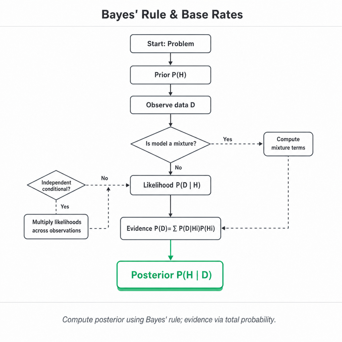
Bayes’ rule is posterior = likelihood × prior / evidence. For hypothesis $H$ and observation $D$ :
$P(H \mid D)=\frac{P(D \mid H)P(H)}{P(D)}$
where $P(D)=\sum_i P(D \mid H_i)P(H_i)$ across mutually exclusive hypotheses. Most mistakes come from ignoring $P(H)$ , the base rate.
Use the law of total probability for mixed populations. If reviewers, users, ads, or chatbot responses come from latent types $T \in \{A,B,C\}$ , compute:
$P(E)=\sum_t P(E \mid T=t)P(T=t)$
This is the backbone of mixture models, fraud/spam classifiers, reviewer quality models, and ads response prediction.
Posterior odds are often cleaner than posterior probabilities. For two hypotheses $H_1,H_2$ :
$\frac{P(H_1 \mid D)}{P(H_2 \mid D)}=\frac{P(H_1)}{P(H_2)} \cdot \frac{P(D \mid H_1)}{P(D \mid H_2)}$
The second term is the likelihood ratio. This is useful when repeated observations accumulate evidence, such as multiple reviewer decisions or repeated chatbot evaluations.
Conditional independence must be stated, not assumed silently. If observations $X_1,\dots,X_n$ are independent conditional on type $T$ , then:
$P(X_1,\dots,X_n \mid T)=\prod_i P(X_i \mid T)$
In Meta-like systems, repeated ratings by the same reviewer, sessions from the same user, or impressions from the same campaign are often correlated.
Linearity of expectation avoids unnecessary joint distributions. Even if events are dependent,
$E\left[\sum_i X_i\right]=\sum_i E[X_i]$
For expected impressions, expected occupied rooms, or expected ads shown, define indicator variables and sum their probabilities. You do not need independence unless computing variance or joint probabilities.
Complements simplify “at least one” probabilities. For independent trials with success probability $p$ :
$P(\text{at least one success in } n)=1-(1-p)^n$
This pattern appears in probability a user receives at least one impression, a chatbot produces at least one bad answer, or an ad gets inserted at least once.
Occupancy problems usually need indicators or multinomial counts. If $m$ items are randomly assigned to $n$ buckets, the probability a specific bucket is empty is $(1-1/n)^m$ , so expected nonempty buckets is $n[1-(1-1/n)^m]$ . For large $m,n$ , use approximations like $(1-1/n)^m \approx e^{-m/n}$ .
Sequential ad-insertion strategies require modeling stopping rules. If ads are inserted after each content item with probability $p$ , counts may follow binomial or geometric-like distributions depending on whether there is a cap, cooldown, or stopping condition. Always clarify whether insertion opportunities are independent, capped, session-length dependent, or adaptive to engagement.
Repeated Bernoulli trials create binomial likelihoods. If $k$ successes occur in $n$ i.i.d. trials,
$P(k \mid p)=\binom{n}{k}p^k(1-p)^{n-k}$
This is central for chatbot quality, reviewer correctness, click outcomes, and pass/fail moderation decisions. For large $n$ , compute in log-space to avoid underflow.
Base rates dominate when signals are weak or rare events are involved. A classifier with 99% sensitivity and 99% specificity can still have poor precision when prevalence is 0.1%. In integrity, harmful content detection, or fake-account review, candidates should distinguish $P(\text{flag} \mid \text{bad})$ from $P(\text{bad} \mid \text{flag})$ .
Exact enumeration does not scale for large state spaces. For a few rooms, reviewer types, or response categories, enumerate all joint states. For thousands or millions of users/items, use indicator expectations, dynamic programming, Poisson/binomial approximations, or Monte Carlo simulation. Exact $2^n$ enumeration is only reasonable for small $n$ .
Check limiting behavior to validate answers. If reviewer accuracy goes to 1, posterior belief should concentrate on the type consistent with observed ratings. If $p=0$ , expected ads should be 0; if $p=1$ , ads should appear at every eligible slot. These sanity checks often catch algebraic inversions.

Worked example

For “Calculate Probabilities for Mixed Reviewer Types,” a strong candidate would first frame it as a latent-type mixture problem: reviewers belong to different reliability groups, each with its own probability of making a correct judgment, and observed reviews update beliefs about which type produced them. In the first 30 seconds, they would ask whether reviewer type is fixed across all decisions, whether decisions are conditionally independent given type, and whether the prior proportions of reviewer types are known. The answer can then be organized around four pillars: define the latent type variable $T$ , write the prior $P(T)$ , specify the likelihood of the observed sequence $P(D \mid T)$ , and normalize using Bayes’ rule to get $P(T \mid D)$ . If the problem asks for an expected future review quality, the candidate should compute a posterior predictive probability: $P(\text{correct next} \mid D)=\sum_t P(\text{correct next} \mid T=t)P(T=t \mid D)$ .

A key tradeoff to flag is whether the model treats observations as independent conditional on reviewer type; this is mathematically convenient but may be unrealistic if reviewers learn, fatigue, copy each other, or face correlated item difficulty. A strong candidate would say, “I’ll assume conditional independence for the calculation, but in production I’d consider item-level random effects or reviewer-item interaction terms.” They would avoid jumping straight into arithmetic before defining events, because the main test is selecting the correct conditioning structure. They would close by checking edge cases: if all observed decisions are correct, the posterior should move toward high-accuracy reviewer types; if the base rate of expert reviewers is tiny, it may still not dominate after only one correct answer. If given more time, they could extend the model to a Beta-Binomial prior over reviewer accuracy rather than a finite set of reviewer types.

A second angle

For “Compare Ad-Insertion Strategies: Expected Ads and Probabilities,” the same probabilistic reasoning applies, but the latent variable may be the user path or session length rather than reviewer type. Instead of updating a posterior over types, you often compute expected counts under different stochastic policies: insert every $k$ items, insert independently with probability $p$ , or insert after a random trigger. The key move is still to define indicator variables for each eligible slot and sum $P(\text{ad at slot } i)$ . If the question asks for “probability of at least one ad,” switch from expectation to complements, e.g. $1-\prod_i P(\text{no ad at slot } i)$ . The product form only holds under independence; if the strategy has cooldowns, caps, or adaptive pacing, the candidate should model the state transition instead of multiplying marginal probabilities.

Common pitfalls

Analytical mistake: confusing inverse conditionals. A tempting wrong answer is to treat $P(\text{good reviewer} \mid \text{correct review})$ as equal to $P(\text{correct review} \mid \text{good reviewer})$ . What lands better is explicitly writing Bayes’ rule and including the denominator, because a rare reviewer type may still have low posterior probability after one good observation.

Communication mistake: doing arithmetic before modeling. Candidates often start multiplying probabilities without saying what is independent, what is conditional, and what the random variables are. A better approach is to define events like $T$ , $D$ , $X_i$ , and state assumptions in one sentence before computing.

Depth mistake: assuming independence in repeated product events. For chatbot quality or repeated ad insertion, it is tempting to say $P(\text{all good})=p^n$ automatically. That only holds for i.i.d. responses; in real systems, prompts from the same topic, ads within the same session, or reviewers seeing similar content can be correlated, requiring conditioning, clustering, or a hierarchical model.

Connections

Interviewers may pivot from this topic into hypothesis testing, A/B experiment interpretation, false discovery rate, calibration of ML classifiers, or precision-recall tradeoffs under class imbalance. They may also ask about Bayesian priors, Beta-Binomial models, Thompson sampling, or how posterior uncertainty affects product decisions like ranking, moderation, and ad allocation.