Probability Modeling, Expectation, And Variance

What's being tested

Interviewers are probing whether you can translate an ambiguous product or experimentation scenario into a probability model, compute expectation or variance correctly, and explain the assumptions behind the math. At Meta, this matters because Data Scientists routinely reason about noisy metrics: click-through rate, conversion, retention, feed engagement, notification opt-outs, ad auction outcomes, and experiment readouts. The interviewer is usually not testing memorized puzzle tricks; they are testing whether you can define random variables, use linearity of expectation, handle dependence, and connect uncertainty to a business decision. Strong answers make the model explicit, quantify uncertainty, and call out where real-world data violates the clean assumptions.

Core knowledge

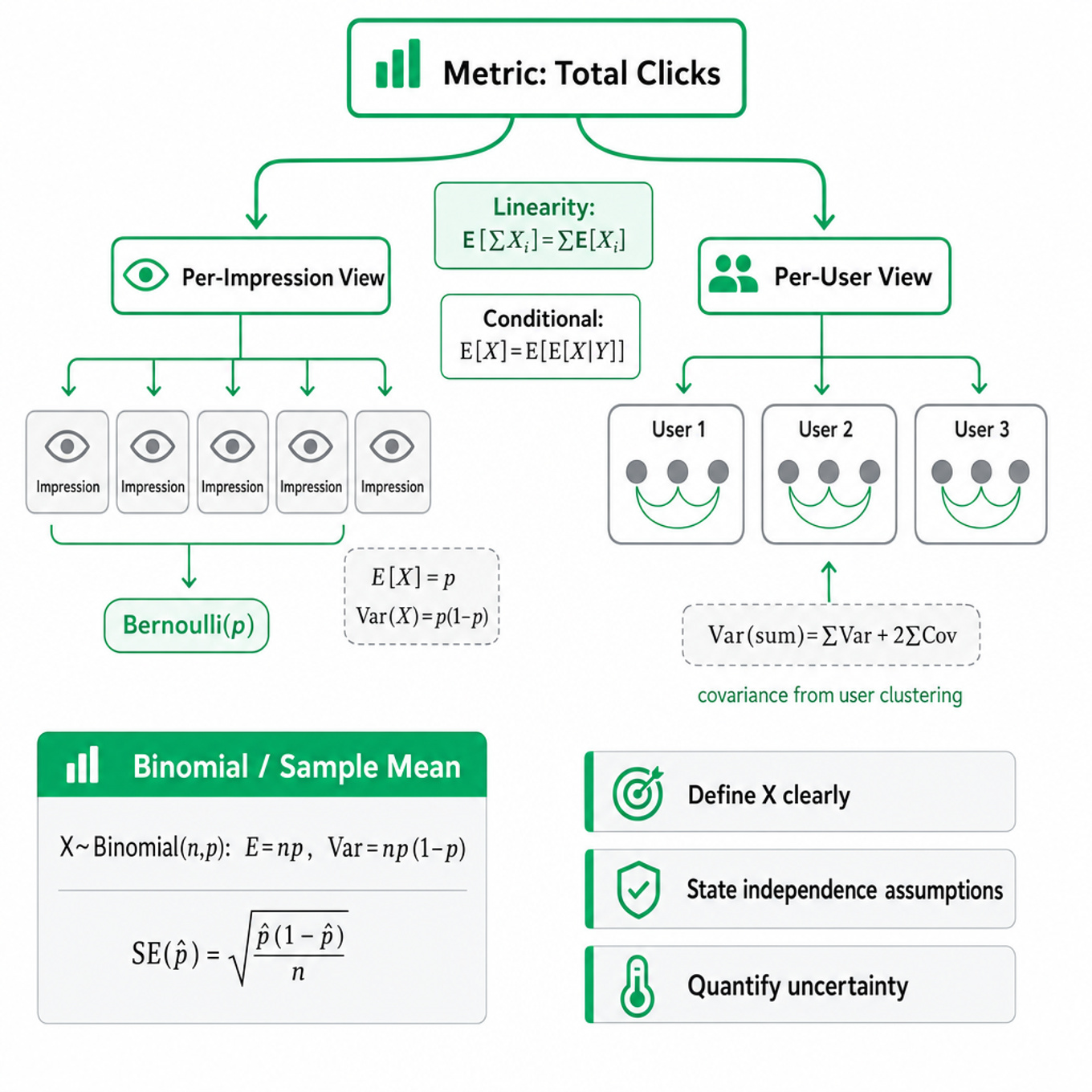
Define the random variable before calculating. For example, if $X$ is “number of users who click,” specify whether users are independent Bernoulli trials, whether click probability is constant, and whether repeated impressions from the same user are allowed.
Expectation is linear even when variables are dependent:
$E\left[\sum_i X_i\right] = \sum_i E[X_i]$
This is extremely useful for counting collisions, active users, clicks, matches, impressions, or expected retained users without modeling the full joint distribution.
Variance is not linear under dependence:
$Var\left(\sum_i X_i\right)=\sum_i Var(X_i)+2\sum_{i<j}Cov(X_i,X_j)$
A common Meta-relevant edge case is user-level clustering: impressions from the same user are correlated, so treating all impressions as independent underestimates uncertainty.
Bernoulli and binomial models are the default for binary outcomes. If $X_i \sim Bernoulli(p)$ , then $E[X_i]=p$ and $Var(X_i)=p(1-p)$ . If $X \sim Binomial(n,p)$ , then $E[X]=np$ and $Var(X)=np(1-p)$ .
The sample mean has expectation $E[\bar X]=\mu$ and variance $Var(\bar X)=\sigma^2/n$ under independent observations. For binary metrics, $SE(\hat p)=\sqrt{\hat p(1-\hat p)/n}$ . At very small or very large $p$ , normal approximations can be poor.
Conditional expectation is often the cleanest path:
$E[X]=E[E[X\mid Y]]$
Use it when the process has stages, such as users receiving notifications, then opening, then clicking. This also helps separate product funnel assumptions.
Bayes’ rule appears in classification, spam/fraud detection, and diagnostic-style interview questions:
$P(A\mid B)=\frac{P(B\mid A)P(A)}{P(B)}$
Always account for the base rate; rare-event settings can produce unintuitive posterior probabilities even with accurate signals.
The law of total variance decomposes uncertainty:
$Var(X)=E[Var(X\mid Y)]+Var(E[X\mid Y])$
This is useful when user segments have different propensities. Segment heterogeneity increases total variance beyond a single pooled-binomial model.
For count data, Poisson approximations work when $n$ is large, $p$ is small, and $\lambda=np$ is moderate: $X \sim Poisson(\lambda)$ , with $E[X]=Var(X)=\lambda$ . This is common for rare clicks, reports, fraud events, or crashes, but overdispersion often appears in real product data.
For occupancy or hashing problems, use indicator variables. If $n$ users are assigned uniformly to $m$ buckets, the expected number of occupied buckets is
$m\left(1-\left(1-\frac{1}{m}\right)^n\right)$
and expected pairwise collisions is $\binom{n}{2}/m$ .
Independence assumptions are the main interview pressure point. Random assignment in A/B tests helps independence between treatment and potential outcomes, but outcomes may still be correlated through social graphs, households, shared advertisers, geography, time, or repeated exposure.
Simulation is acceptable as a validation tool, not a substitute for modeling. For small state spaces, exact enumeration or dynamic programming may be feasible; for millions of users or complex funnels, Monte Carlo simulation can sanity-check expectation and variance under explicit assumptions.

Worked example

Expected Number of Collisions When Hashing Users Into Buckets

A strong candidate would first clarify the setup: “Are users assigned independently and uniformly at random to buckets? Do we care about pairwise collisions, buckets with at least two users, or the number of users involved in a collision?” Those are different random variables, so the first 30 seconds should be spent defining the target clearly. The answer can be organized around four pillars: define indicators, compute expectation for one indicator, sum using linearity of expectation, then discuss assumptions and edge cases. For pairwise collisions, the natural indicator is $I_{ij}=1$ if users $i$ and $j$ land in the same bucket, and $E[I_{ij}]=1/m$ under uniform hashing. Then the expected total number of colliding pairs is the sum over all $\binom{n}{2}$ pairs; no independence between indicators is required for expectation.

The candidate should explicitly flag a tradeoff: pairwise collisions are easy to compute, but they are not the same as “number of buckets with collisions” or “number of users affected,” which require different indicators. If the interviewer pushes toward variance, the candidate should note that covariance terms matter because collision indicators sharing a user are not automatically independent in all variants of the problem. A Meta-style business connection would be bucket assignment for experiments, cache keys, ranking shards, or holdout groups, where non-uniform hashing could bias traffic or overload systems. A good close would be: “If I had more time, I’d verify the uniformity assumption empirically by checking bucket counts with a chi-square test and looking for user attributes correlated with bucket assignment.”

A second angle

Variance of a Click-Through Rate Estimate

The same modeling skill applies, but the framing shifts from counting expected events to quantifying uncertainty around a metric. If each user has one impression and click outcome $X_i \sim Bernoulli(p)$ , then the CTR estimate $\hat p=\frac{1}{n}\sum_i X_i$ has variance $p(1-p)/n$ . However, if users receive multiple impressions, treating impressions as independent is often wrong because the same user’s clicks are correlated. A stronger model aggregates at the user level or uses cluster-robust standard errors. The key transfer is the same: define the random variable, state independence assumptions, compute expectation or variance, and explain where the simplified model may break in production data.

Common pitfalls

Analytical mistake: assuming independence when only linearity is needed.
Candidates often say “we can sum these because the events are independent,” even when independence has not been established. For expectation, say “linearity of expectation applies regardless of dependence”; for variance, explicitly check covariance terms instead of silently dropping them.

Communication mistake: solving before defining the random variable.
A tempting but weak answer starts writing formulas immediately: $np$ , $p(1-p)$ , or $\binom{n}{2}/m$ . A better answer first says what $X$ measures, what one trial is, what assumptions are being made, and whether the desired output is an expectation, a probability, or a confidence interval.

Depth mistake: giving a toy answer without production caveats.
For a binary metric, “variance is $p(1-p)/n$ ” is correct only under independent Bernoulli observations. In Meta-scale data, repeated exposure, network effects, bot traffic, segment heterogeneity, logging delays, and experiment interference can dominate the theoretical variance if ignored.

Connections

Interviewers can easily pivot from this topic into A/B testing, confidence intervals, power analysis, sequential testing, or causal inference. They may also connect probability modeling to metric design, ranking evaluation, ads auction modeling, anomaly detection, or Bayesian updating for rare events.