Probability Models and Poisson Approximations
Asked of: Data Scientist
Last updated
-
What it is Probability models describe randomness with mathematical structures (e.g., Bernoulli, Binomial, Poisson). When events are rare and mostly independent, the Poisson distribution models their counts over time/space; the Poisson approximation replaces a harder count model (often Binomial or Poisson-binomial) with a Poisson having mean λ equal to the expected count.
-
Why interviewers ask about it Data Scientists at companies like Meta routinely analyze low-rate events: crashes per user-day, spam flags per thousand messages, or rare conversions. Knowing when a Binomial can be approximated by a Poisson, and when to prefer Poisson/Negative Binomial regression, helps you size experiments, compute tail risks, and reason quickly about capacity and anomaly alerts.
-
Core ideas to know
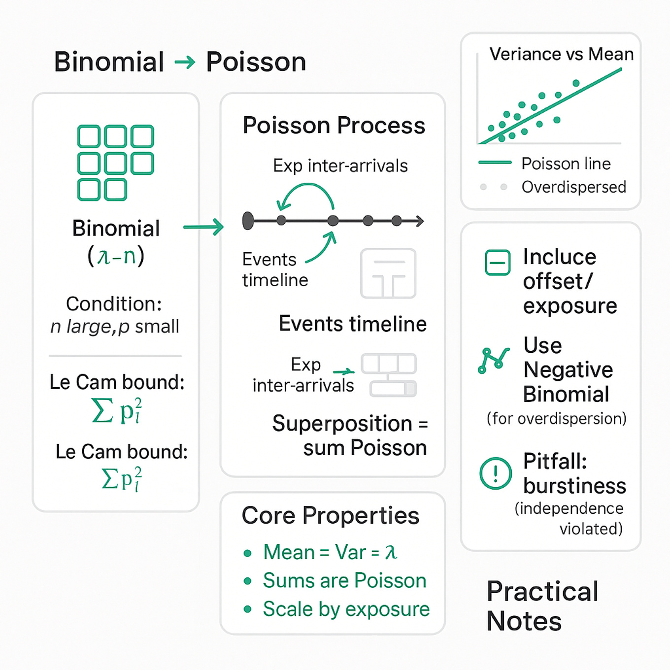
- Poisson models counts of independent, rare events in fixed exposure; mean equals variance: E[X] = Var[X] = λ.
- Approximate Binomial(n, p) with Poisson(λ = np) when n is large and p is small.
- Le Cam’s theorem gives a total-variation error bound proportional to ∑ p_i^2 for rare events.
- Superposition: sums of independent Poisson variables are Poisson; thinning a Poisson with rate q gives Poisson(qλ).
- Inter-arrival times are Exponential; the Poisson process is memoryless; always scale by exposure (time, users, area).
- Overdispersion breaks Poisson; consider Negative Binomial or quasi-Poisson and include offsets/exposure.
- Poisson regression (GLM with log link) models counts given features; use an offset to handle varying exposure.
-
A common pitfall Candidates often invoke a Poisson model without checking independence or rarity. Bursty traffic (bots, outages) violates assumptions, inflating variance and making Poisson confidence intervals too tight. Another failure mode is forgetting exposure: comparing raw counts across regions or app versions instead of counts per user-hour. Finally, defaulting to Poisson when zero-inflation or heavy tails demand Negative Binomial leads to biased inferences and brittle alerts.
-
Further reading
- Mitzenmacher & Upfal — Probability and Computing (2nd ed., Cambridge): Clear, CS-focused treatment of Poisson approximation, balls-into-bins, hashing, and the Poisson process. (assets.cambridge.org)
- Blitzstein & Hwang — Introduction to Probability (2nd ed., Routledge): Intuitive coverage connecting Binomial↔Poisson and Poisson processes, with practical examples and exercises. (routledge.com)
- scikit-learn PoissonRegressor: Practical GLM for count data (log link, offsets, regularization); a useful production counterpart to the theory. (sklearn.org)