SQL Event Analytics

What's being tested

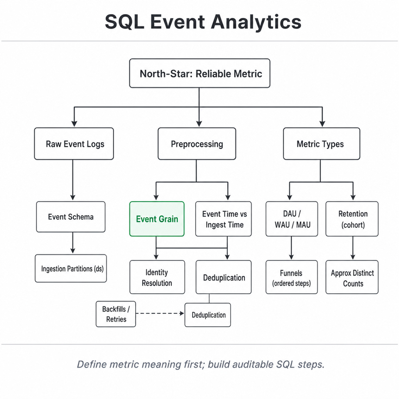
Meta-style event analytics SQL tests whether you can turn raw product logs into trustworthy behavioral metrics under realistic data conditions. Interviewers are probing more than syntax: they want to see if you understand event grain, user identity, time windows, deduplication, joins, and metric definitions well enough to avoid misleading results. The strongest answers clarify the business meaning of the metric before writing SQL, then build the query in auditable steps. This matters because Meta product decisions often depend on high-volume event streams where a small counting or attribution error can change conclusions about growth, engagement, or product quality.

Core knowledge

• Event tables are usually append-only logs with fields like user_id, event_name, event_time, event_date, session_id, device_id, and metadata JSON. Always identify the grain: one row per event, per impression, per click, per message, or per state transition.

• Distinguish event time from processing time. event_time is when the user action happened; ds, event_date, or partition date may reflect ingestion time. For behavioral metrics, use event time, but filter partitions for performance, e.g. WHERE ds BETWEEN ... plus event_time constraints.

• DAU, WAU, and MAU are distinct-user metrics:
  $DAU_d = COUNT(DISTINCT user_id \text{ active on day } d)$
  Define “active” explicitly: app open, feed view, session start, message send, or any logged event can produce very different numbers.

• Retention is cohort-based and requires a starting event plus a return event. Day-$N$ retention is usually:
  $\frac{\text{users in cohort with activity on cohort\_date + N}}{\text{users in cohort}}$
  Avoid counting multiple returns per user by aggregating to one row per user-cohort before computing rates.

• Funnel analysis requires step ordering. For signup → profile creation → first friend add, ensure each later event occurs after the previous event, often using MIN(CASE WHEN ...) per user or window functions. Counting users who ever did each step overstates conversion.

• Use COUNT(DISTINCT user_id) carefully at Meta scale. Exact distinct counts can be expensive for billions of rows; approximate methods like HyperLogLog via approx_distinct() are common when small error, often ~1–2%, is acceptable for exploratory analysis.

• Deduplication is essential when events can be retried, backfilled, or emitted by multiple clients. Prefer a stable event_id or idempotency key. If unavailable, dedupe using a composite such as user_id, event_name, event_time, and key metadata, while acknowledging collision risk.

• Window functions are central: ROW_NUMBER() for deduping or first event, LAG() for inter-event gaps, SUM() OVER for running totals, and MIN() OVER for first-touch attribution. Always specify deterministic ordering when ties are possible.

• Sessionization usually defines a new session after inactivity, commonly 30 minutes: new_session = gap_minutes > 30. Use LAG(event_time) per user, then cumulative sum to assign session IDs. Edge cases include cross-device activity and background pings.

• Joins can silently change counts. Joining an event table to a many-row dimension table can multiply events. Before joining, check dimension uniqueness at the join key, or aggregate the dimension to one row per key using ROW_NUMBER() or MAX_BY().

• Time zones matter for daily metrics. Meta-scale products often report in UTC for consistency, but business teams may need local user days. A user active at 23:30 PST and 00:30 UTC can fall into different “days” depending on the definition.

• Late-arriving data and backfills affect dashboards. A metric for yesterday may be incomplete if mobile clients upload logs hours later. Good answers mention data freshness, watermarking, and whether the metric should use a fixed lookback buffer, such as waiting 24–48 hours before finalizing retention.

Worked example — “Calculate 7-day retention by signup cohort”

A strong candidate would start by clarifying the cohort and return definitions: “Is the cohort based on first signup date, account creation date, or first app open, and does 7-day retention mean activity exactly on day 7 or any activity within days 1 through 7?” They would also ask whether to use UTC or user-local dates, and whether deleted, test, or banned accounts should be excluded. The answer skeleton should have four pillars: build a clean signup cohort with one row per user, build a clean activity table with one row per user per active date, join cohort users to activity on the target retention date, and aggregate by cohort date.

The SQL would likely use a CTE for cohort with MIN(signup_time) per user, another CTE for activity filtered to qualifying active events, and then a LEFT JOIN so non-retained users remain in the denominator. The candidate should explicitly avoid an INNER JOIN as the main retention join, because it drops non-returning users and makes the denominator equal only to retained users. A precise definition might be: exact D7 retention where activity_date = signup_date + INTERVAL '7' DAY; rolling D7 would instead use activity_date BETWEEN signup_date + 1 AND signup_date + 7. One tradeoff to flag is exact distinct counting versus pre-aggregating user-day activity: pre-aggregation reduces row volume and join cost while preserving correctness for retention. A good close would be: “If I had more time, I’d validate counts against known signup totals, inspect late-arriving data sensitivity, and segment by platform or acquisition channel to identify where retention differs.”

A second angle — “Compute daily active users and 7-day rolling active users”

The same skills apply, but the metric is no longer cohort-based; it is calendar-window based. For DAU, the query can aggregate qualifying events to one row per user_id, activity_date, then count distinct users per day. For 7-day rolling active users, the candidate must count users active at least once in the trailing 7-day window, not sum seven DAU values, because the same user can be active on multiple days. The SQL might join a date spine to user-day activity where activity_date BETWEEN report_date - INTERVAL '6' DAY AND report_date, then count distinct users per report date. The key constraint changes from preserving a cohort denominator to correctly handling overlapping windows and avoiding double-counting.

Common pitfalls

An analytical mistake is treating event rows as users. A tempting but wrong query is COUNT(*) WHERE event_name = 'app_open' and calling it DAU; this counts active events, not active users. A better answer defines the user-level unit first and uses COUNT(DISTINCT user_id) or pre-aggregates to one row per user-day.

A communication mistake is jumping straight into SQL without confirming metric semantics. For example, “7-day retention” can mean exact day 7, any return within 7 days, or return during the second week. Strong candidates state assumptions explicitly and explain how the query would change under alternate definitions.

A depth mistake is ignoring production data issues. Interviewers may push on duplicate events, late logs, missing user IDs, bot/test traffic, or timezone boundaries. Saying “the table is clean” is weak; it is better to say “assuming the upstream table is deduped; otherwise I’d dedupe by event_id using ROW_NUMBER() before computing the metric.”

Connections

Interviewers often pivot from event analytics SQL into experimentation, especially how to compute experiment metrics from event logs without post-treatment bias. They may also ask about metric design, funnel diagnostics, retention curves, causal interpretation, or scalable data infrastructure using Hive, Presto, Spark, and partitioned tables. If the discussion turns to correctness under noisy logging, expect follow-ups on data quality checks, instrumentation design, and identity resolution.

Further reading

• Designing Data-Intensive Applications — Strong foundation for event logs, distributed data systems, late data, and correctness tradeoffs.
• The Data Warehouse Toolkit by Ralph Kimball and Margy Ross — Useful for understanding fact table grain, dimensions, and analytical modeling.
• Presto Documentation — Practical reference for SQL functions commonly used in large-scale event analytics, including window functions and approximate aggregations.