SQL Joins, Aggregation, And Window Functions

What's being tested

Interviewers are testing whether you can translate messy product data into correct, efficient metrics using SQL, not whether you can memorize syntax. At Meta, Data Scientists work with event logs, user tables, experiment assignments, ads/impression tables, and social graph data where joins can silently change the unit of analysis. The interviewer is probing whether you understand grain, fanout, missing data, deduplication, and time-based aggregation well enough to produce trustworthy numbers. Strong answers show both correctness and practical judgment: you can explain why a query returns the metric the business asked for, and how you would make it scalable on large tables.

Core knowledge

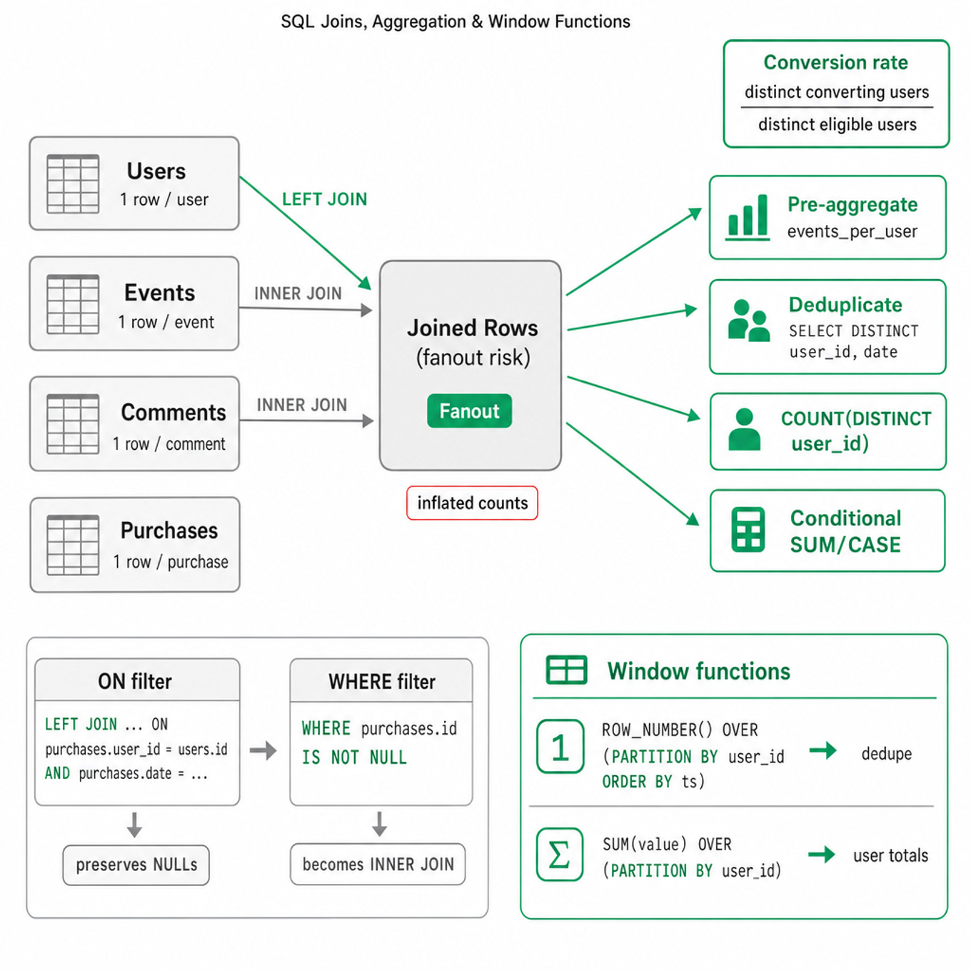
Always identify the grain of every table before writing SQL: one row per user, event, session, impression, message, or user-day. Most SQL mistakes come from joining tables at incompatible grains, causing fanout and inflated counts, sums, or averages.
Know the join types and their metric implications. INNER JOIN keeps only matched records; LEFT JOIN preserves the left table; FULL OUTER JOIN is useful for reconciliation; CROSS JOIN intentionally creates combinations. In product analytics, LEFT JOIN is common when measuring non-conversion or inactive users.
Be careful where you place filters after outer joins. A condition like WHERE purchases.purchase_id IS NOT NULL after a LEFT JOIN turns it into an inner join. Put right-table filters in the ON clause when you want to preserve unmatched left-side rows.
Diagnose fanout explicitly. If users joins to events and events joins to comments, then one user can become many rows. Use pre-aggregation, COUNT(DISTINCT user_id), or join on a deduplicated subquery such as SELECT DISTINCT user_id, date FROM events.
Aggregation requires matching numerator and denominator grains. Conversion rate is usually $\frac{\text{distinct converting users}}{\text{distinct eligible users}}$ not AVG(converted) over event rows unless each user contributes exactly one row. Declare whether the denominator is users, sessions, impressions, or days.
Conditional aggregation is a standard pattern: SUM(CASE WHEN condition THEN 1 ELSE 0 END) for counts, COUNT(DISTINCT CASE WHEN condition THEN user_id END) for unique users, and AVG(CASE WHEN condition THEN value END) for conditional means. Avoid COUNT(CASE WHEN ... THEN 0 END) because non-null zeros are counted.
Window functions compute values across related rows without collapsing the result set. Common patterns: ROW_NUMBER() for deduplication, RANK()/DENSE_RANK() for leaderboards, LAG()/LEAD() for previous-event comparisons, and SUM(x) OVER (PARTITION BY user_id ORDER BY ds) for cumulative metrics.
Understand window frames. ORDER BY ds with SUM() OVER may default to a RANGE frame in some SQL engines, grouping tied timestamps. Use explicit frames like ROWS BETWEEN 6 PRECEDING AND CURRENT ROW for 7-row rolling windows or date filters for true 7-day calendar windows.
Top-N queries usually require windows, not just ORDER BY ... LIMIT. To get top 3 posts per country, compute ROW_NUMBER() OVER (PARTITION BY country ORDER BY impressions DESC) and filter WHERE rn <= 3. Use RANK() if ties should share placement.
Deduplication is a recurring Meta-style theme because event logs can contain retries, duplicate sends, and late arrivals. Use a stable event identifier when available; otherwise use ROW_NUMBER() OVER (PARTITION BY user_id, event_type, timestamp ORDER BY ingestion_time DESC) and keep rn = 1.
SQL execution order matters: FROM/JOIN, WHERE, GROUP BY, HAVING, window functions, SELECT, ORDER BY, LIMIT conceptually happen in stages. Since windows are evaluated after aggregation in many dialects, complex metrics often need CTEs to separate row-level, aggregate-level, and window-level logic.
Performance matters on event-scale data. Partition prune on date columns, filter early, select only needed columns, pre-aggregate before joining high-cardinality tables, and avoid unnecessary COUNT(DISTINCT ...) on billions of rows. At very large scale, systems may use HyperLogLog-style approximate distinct counts with small relative error.

Worked example

Daily Active Users by Country

A strong candidate would first clarify the definition: “Does active mean any app event, a session start, feed view, or a qualifying action? Should country come from the user profile, event IP, or latest known location? What timezone defines the day?” They would also establish the desired grain: one output row per date, country, counting distinct users active on that date. The answer should be organized around four pillars: define the eligible events, deduplicate to one row per user_id, date, join to a country source at the correct time grain, then aggregate distinct users by date and country.

The skeleton query would likely use a CTE such as active_user_days with SELECT DISTINCT user_id, DATE(event_time) AS ds FROM events WHERE event_type IN (...), followed by a join to a user or location table. If the country table has multiple rows per user over time, the candidate should avoid a naive join and instead choose the country valid at the event date, often with ROW_NUMBER() over location records or an effective-date join. A specific tradeoff to flag is whether to use COUNT(DISTINCT user_id) directly on raw events versus pre-deduplicating user-days first; pre-deduplication is safer for avoiding fanout and often cheaper when joined downstream. The candidate should mention edge cases: null country, deleted users, bots/internal traffic, late-arriving events, and users who travel during the day. A strong close would be: “If I had more time, I’d validate the query by comparing total DAU before and after the country join, checking for fanout, and reconciling against a trusted metrics table.”

A second angle

7-Day Rolling Retention

The same concepts apply, but the framing shifts from counting activity to comparing a cohort against future behavior. A candidate should define the cohort grain first, usually one row per user signup date or first active date, then join or window over future activity dates to determine whether the user returned within days 1 through 7. The main risk is double-counting users who return multiple times, so the query should reduce activity to distinct user_id, active_date before computing retention. A window function can help find the first activity date with MIN(active_date) OVER (PARTITION BY user_id), while conditional aggregation computes retained users by cohort. Unlike DAU, the denominator is fixed at cohort creation time, so using only users who have later events would bias the retention rate upward.

Common pitfalls

Analytical mistake: ignoring fanout. A tempting wrong answer is to join users to events to purchases and then run COUNT(user_id) or SUM(revenue) without checking row multiplication. A better answer states the grain after each join and pre-aggregates purchases or events before joining, then validates that row counts behave as expected.

Communication mistake: writing SQL before defining the metric. Candidates often jump straight into SELECT date, COUNT(DISTINCT user_id) without clarifying “active,” timezone, denominator, or whether bots/test users are excluded. At Meta, the interviewer wants to see metric ownership: define assumptions aloud, then write SQL consistent with those assumptions.

Depth mistake: using window functions mechanically. ROW_NUMBER() is powerful, but using it without explaining tie-breakers can produce nondeterministic results. If two records have the same timestamp, specify a stable secondary order such as ORDER BY event_time DESC, ingestion_time DESC, event_id DESC, and explain why that row should win.

Connections

Interviewers can pivot from this topic into metric design, experimentation analysis, data quality, and product sense. Expect follow-ups on cohort retention, A/B test guardrail metrics, logging reliability, Simpson’s paradox in aggregated metrics, or approximate counting methods such as HyperLogLog.