SQL Joins, Aggregations, And Window Functions

What's being tested

Interviewers are testing whether you can translate a product or logging question into correct relational logic under messy real-world data conditions. For Meta Data Scientist roles, SQL is not just syntax: it is how you define metrics, debug data quality, evaluate experiments, and reason about user behavior at massive scale. The interviewer is probing whether you understand join grain, aggregation level, deduplication, null handling, and windowed ranking over event streams. Strong candidates make assumptions explicit, choose the right unit of analysis, and avoid producing a query that “runs” but answers the wrong business question.

Core knowledge

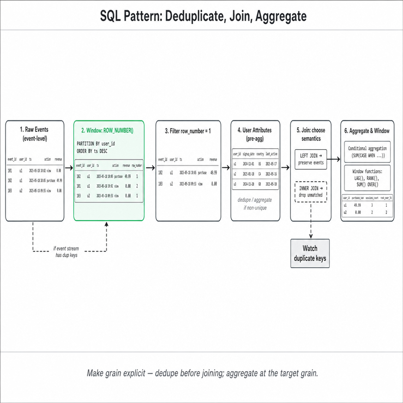
Always identify the grain before writing SQL: one row per user, event, session, request, day, or user-day. Most SQL interview mistakes come from mixing grains, such as joining event-level impressions to user-level attributes and then counting users after duplication.
Know join semantics precisely. INNER JOIN keeps matched rows only; LEFT JOIN preserves the left table and fills unmatched right columns with NULL; FULL OUTER JOIN preserves both sides; CROSS JOIN creates $N \times M$ rows and is usually only intentional for date spines or parameter grids.
Join keys are rarely perfectly unique. Before joining, ask whether the right table has one row per key. If not, pre-aggregate or deduplicate with ROW_NUMBER(); otherwise metrics like revenue, sessions, or comments can inflate multiplicatively.
Use conditional aggregation for segmented metrics: SUM(CASE WHEN condition THEN 1 ELSE 0 END), COUNT(CASE WHEN condition THEN id END), and AVG(CASE WHEN condition THEN value END). For rates, write numerator and denominator explicitly: $\text{rate}=\frac{\text{eligible successes}}{\text{eligible opportunities}}$ .
COUNT(*), COUNT(column), and COUNT(DISTINCT column) mean different things. COUNT(*) counts rows, including nulls; COUNT(column) ignores nulls; COUNT(DISTINCT user_id) deduplicates but may be expensive at Meta-scale. Approximate distinct algorithms like HyperLogLog are often used for very large cardinalities.
Window functions operate after FROM, WHERE, GROUP BY, and HAVING, but before the final ORDER BY. Common patterns: ROW_NUMBER() for deduplication, RANK() / DENSE_RANK() for leaderboards, LAG() / LEAD() for prior events, and windowed SUM() for cumulative metrics.
Understand window frames. ROWS BETWEEN 6 PRECEDING AND CURRENT ROW means seven physical rows, not necessarily seven calendar days. For date-based rolling windows, first build a complete date spine or use range-aware logic if the SQL engine supports it.
Choose the right ranking function. ROW_NUMBER() breaks ties arbitrarily unless fully ordered; RANK() leaves gaps after ties; DENSE_RANK() does not. For “top 3 users including ties,” RANK() <= 3 differs from “exactly three rows,” which usually needs ROW_NUMBER() <= 3.
Be careful with filters on outer joins. A LEFT JOIN followed by WHERE right_table.status = 'accepted' effectively becomes an inner join. Put right-side filters in the ON clause or use conditional aggregation if unmatched rows must remain in the denominator.
Time boundaries matter. Product data is usually timestamped in UTC, while metrics may be reported by local day or Pacific Time. Use half-open intervals like event_ts >= start_ts AND event_ts < end_ts instead of BETWEEN, especially for daily, weekly, and experiment windows.
For large event tables, performance depends on partition pruning, pre-aggregation, and avoiding unnecessary COUNT(DISTINCT). In Hive/Presto/Trino-style systems, filter partition columns early, aggregate before joining when possible, and avoid joining two raw multi-billion-row fact tables directly.
Nulls are not zeros. In arithmetic, NULL propagates; in joins, null keys do not match; in averages, nulls are skipped. Use COALESCE() deliberately, but only after deciding whether missing data means zero activity, unknown activity, or ineligible population.

Worked example

For “Comments Distribution”, a strong candidate would start by clarifying the metric: “Are we calculating the distribution of number of comments per user over a fixed time window, and should users with zero comments be included?” They would also ask whether deleted comments, bot users, or duplicate comment events should count, and what timestamp defines inclusion. The first pillar of the answer is grain: create one row per user with their comment count during the period. The second pillar is join strategy: start from the user population if zero-comment users belong in the distribution, then LEFT JOIN comments filtered to the target window. The third pillar is aggregation: first aggregate comments by user, then aggregate users by comment count to produce buckets such as 0 comments -> N users, 1 comment -> N users, and so on.

A skeleton answer would use a CTE for eligible users, a CTE for comments in the date range, a CTE that counts comments per user, and a final GROUP BY comment_count. The main tradeoff to flag is whether to join raw comments to users first or pre-aggregate comments first; pre-aggregating usually reduces data volume and avoids user rows being duplicated unnecessarily. They should explicitly mention that filtering comments in the WHERE clause after a left join would drop zero-comment users, so the date filter belongs inside the comments CTE or the join condition. A strong close would be: “If I had more time, I’d validate the distribution against total comments and total eligible users, and check whether spam/deleted comments or timezone boundaries change the result.”

A second angle

For “Friend Request Acceptance Rate”, the same ideas apply, but the central challenge is denominator definition rather than distribution construction. The candidate must decide whether the denominator is all sent requests, unique requester-recipient pairs, or only requests that had enough time to be accepted. A clean solution usually deduplicates request events and accept events separately, joins accepts back to sends on requester, recipient, and possibly request date, then computes accepted_requests / sent_requests. The join type matters: using an INNER JOIN would count only accepted requests and produce a misleading 100% acceptance rate. A window function may be needed if multiple requests occur between the same pair, for example to match the first acceptance after the most recent send.

Common pitfalls

An analytical mistake is aggregating at the wrong level, such as counting comments after joining to a user attributes table with multiple historical rows per user. The tempting query may return plausible numbers but inflate active users or comments. A better answer first enforces one row per entity at the intended grain, then joins.

A communication mistake is jumping directly into SQL without clarifying numerator, denominator, population, and time window. Meta interviewers often care less about memorized syntax than whether the candidate can turn an ambiguous product question into a defensible metric. Say your assumptions out loud before coding.

A depth mistake is knowing window function syntax but not tie behavior or frame semantics. For example, using ROW_NUMBER() for “top creators” without specifying deterministic tie-breakers can make results unstable across runs. A stronger answer states whether ties should be included and chooses RANK(), DENSE_RANK(), or ROW_NUMBER() accordingly.

Connections

Interviewers may pivot from SQL mechanics to metric design, experimentation, data quality, or product analytics. Expect follow-ups on retention cohorts, funnel conversion, Simpson’s paradox in segmented aggregates, or how to validate a query against source-of-truth dashboards. For more infrastructure-oriented loops, they may ask about partitioning, approximate distinct counting, or why a query is slow in Presto/Hive.