Airbnb Data Scientist Interview Prep Guide

Focus most on A/B testing, causal inference, metric design, power/MDE, experiment diagnostics, unit-of-randomization/interference, and two-sided marketplace experiments because you rated Analytics & Experimentation 1/5 and selected those exact gaps. You're stronger on Data Manipulation at 4/5, so SQL/Python gets lighter coverage except for window functions and experiment-ready exposure/event-log construction. The Airbnb-specific emphasis is search ranking and guest-host matching, trust/review integrity, and dynamic pricing/host supply elasticity. With less than a week left, this plan budgets about 70 minutes for a focused cheatsheet pass, with most time spent on emphasized experiment and marketplace concepts.

Technical Screen — 70 min

Analytics & Experimentation

Focus area — You rated this shaky and selected A/B testing, power, diagnostics, delayed outcomes, and marketplace experiment threats as focus areas.

What's being tested

The interviewer is probing your ability to design and analyze rigorous randomized experiments that support causal claims in a marketplace. Expect to demonstrate clear estimand formulation, principled choice of randomization unit, power/sample-size calculation (including clustering), handling noncompliance and contamination, and an analysis plan that includes quality checks and variance reduction. Airbnb cares because experimental decisions affect hosts and guests asymmetrically and can produce platform-level externalities; the interviewer wants to see statistical rigor plus product-aware tradeoffs.

Core knowledge

• Estimand: clearly state the causal quantity (e.g., Intent-to-Treat (ITT) lift, Complier Average Causal Effect (CACE)), and how it maps to assignment vs. exposure signals in logs.

• Randomization unit: choose between user-level, listing-level, host-level, or cluster-randomization by weighing contamination risk, statistical power, and operational feasibility.

• Sample-size / power: for a difference in means, use $n=\frac{(Z_{1-\alpha/2}+Z_{1-\beta})^2 2\sigma^2}{\delta^2}$ and multiply by design effect $DE=1+(m-1)\rho$ for clustered designs.

• Clustering & ICC: estimate intraclass correlation (ICC) from historical data; even small $\rho$ inflates required sample when cluster size $m$ is large.

• Noncompliance & IV: analyze assignment-based ITT as primary; use instrumental variable (IV) to estimate CACE: $CACE=\frac{\text{ITT}}{\text{compliance rate}}$ under monotonicity and exclusion assumptions.

• Contamination & interference: when SUTVA fails, consider exposure mapping, partial interference assumptions, or cluster randomization; anticipate bias toward the null from spillovers.

• Sequential testing: pre-specify look schedule and use alpha-spending (O’Brien–Fleming / Pocock) or adjust via group-sequential methods; otherwise control Type I inflation.

• Variance reduction: use covariate adjustment (ANCOVA) or CUPED with pre-experiment covariates to increase power without inflating Type I error.

• Metrics & guardrails: pick one primary metric (business-significant, measurable), plus diagnostic and safety/guardrail metrics (e.g., booking_rate, latency, refund_rate) and define exact aggregations (user-level vs. session-level).

• Integrity checks: log and monitor Sample Ratio Mismatch (SRM), assignment fidelity, treatment exposure rates, and delayed-event completeness; run A/A tests to validate pipeline.

• Multiple comparisons: when testing many segments or metrics, control false discovery (Bonferroni, Benjamini–Hochberg) or pre-specify hierarchical testing to preserve power.

• Practical data signals: derive assignment from reliable sources (treatment_assignment table or randomization seed), and define exposure windows and eligibility consistently to avoid immortal-time bias.

Tip: always declare the primary estimand, the unit of analysis, and the stopping rule within the first minute of your plan.

Worked example — Design and Analyze Airbnb Locker Experiment

Start by clarifying scope: who is eligible (guests, hosts, or listings), operational constraints (number of lockers, geographies), and the timescale for bookings vs. locker use. Organize the answer around 4 pillars: (1) estimand (e.g., effect on booking_rate per exposed guest — ITT), (2) randomization (likely listing- or neighborhood-cluster randomization to avoid contamination between co-located guests), (3) metrics, power, and sample size (compute detectable lift for expected baseline booking rate, inflate by design effect), and (4) analysis & diagnostics (ITT primary, per-protocol secondary; SRM checks; covariate adjustment using historical booking propensity). A key tradeoff: listing-level assignment reduces contamination but increases ICC and sample requirements; user-level assignment has more power but higher spillover risk if guests see lockers tied to listings. Close by proposing guardrails (cancellation_rate, host_response_time) and by saying "if I had more time I’d precompute ICC from historical neighborhood cohorts, run an A/A, and simulate power under several contamination scenarios."

A second angle — Design a network-aware Wi‑Fi badge experiment

This problem foregrounds interference: badges on the same network create spillovers. Frame the estimand as an exposure-conditional causal effect (e.g., effect on engagement for users whose router has >=1 treated badge). Consider partial interference by treating networks (or access points) as independent clusters and randomizing at the network-level. Use exposure mapping to define treatment levels (0,1,≥2 badges) and estimate dose–response or pairwise contrasts. Analysis methods include cluster-randomized inference, permutation tests respecting network blocks, and regression with network-size controls. Explicitly discuss how increasing cluster size inflates sample needs via the design effect and how to detect violations by checking cross-network traffic or attribute overlap.

Common pitfalls

Pitfall: Ignoring clustering — designers often compute sample size as if observations are independent; forgetting the ICC leads to underpowered experiments and misleadingly small p-values. Always estimate and apply the design effect.

Pitfall: Vague estimand and unit of analysis — saying “improve bookings” without specifying ITT vs. treated-exposed, or user- vs. listing-level aggregation, makes results uninterpretable; state aggregations and denominators precisely.

Pitfall: Uncontrolled peeking and multiple looks — analysts run mid-test checks without pre-specified stopping rules; this inflates Type I error. Either lock the look schedule or use alpha-spending/group-sequential methods and record all interim analyses.

Connections

Interviewers may pivot to observational causal inference (propensity scores, DiD) when experiments are infeasible, or to uplift modeling for heterogeneous treatment effect estimation. They might also ask about metric design for recommender evaluation or ML model evaluation metrics (AUC, calibration) as extensions.

Further reading

• Trustworthy Online Controlled Experiments: A Practical Guide to A/B Testing — Kohavi et al., Microsoft-style handbook with practical checks and examples.

• Imbens, G., & Rubin, D., "Causal Inference for Statistics, Social, and Biomedical Sciences" — rigorous treatment of IV, compliance, and potential outcomes.

Practice questions

Focus area — You marked causal inference new and selected observational causal inference, so start from estimands, confounding, counterfactuals, and quasi-experiment logic.

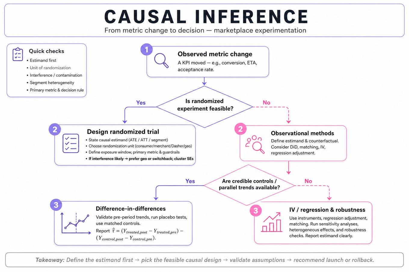
What's being tested

DoorDash causal inference interviews test whether you can move from “a metric changed” to “what caused it, how would we prove it, and what decision should we make?” The interviewer is probing for marketplace experimentation, counterfactual reasoning, metric design, and structured diagnosis across consumers, merchants, and Dashers. DoorDash cares because small operational changes—pay models, batching, merchant selection, grocery substitution flows, ETA promises—can shift multiple sides of the marketplace at once. A strong Data Scientist distinguishes correlation from causation, chooses the right unit of analysis, anticipates interference, and translates evidence into a launch or rollback recommendation.

Core knowledge

• Causal estimand comes before method. State whether you need the average treatment effect: $ATE = E[Y(1) - Y(0)]$, treatment effect on treated, local effect, or segment-specific effect. For DoorDash, effects often differ by market, daypart, merchant type, weather, and order distance.

• Randomized controlled trials are the gold standard when feasible. Define treatment, control, randomization unit, exposure window, primary metric, guardrails, and decision rule upfront. Common units include consumer, merchant, Dasher, delivery, store, or geo-market; the wrong unit can create contamination.

• Interference is central in marketplaces. One Dasher’s incentive treatment can affect untreated consumers through supply reallocation, batching, and ETA changes, violating SUTVA. If spillovers are likely, prefer geo-level randomization, switchback designs, or explicit network/market-level analysis over naive user-level randomization.

• Switchback experiments work well for operational levers that affect a market in real time, such as Dasher pay, dispatch logic, or batching. Randomize market-time blocks, for example city-hour or zone-daypart, and analyze with clustered standard errors. Watch for carryover effects if incentives alter Dasher positioning after the treatment block.

• Difference-in-differences estimates causal effects when randomization is unavailable:
  $\hat{\tau} = (Y_{treated,post} - Y_{treated,pre}) - (Y_{control,post} - Y_{control,pre})$
  Its key assumption is parallel trends. Validate with pre-period trend plots, placebo tests, and matched controls before trusting the estimate.

• Regression adjustment improves precision but does not magically remove bias. A model like $Y_i = \alpha + \beta T_i + \gamma X_i + \epsilon_i$ is credible when treatment assignment is as-good-as-random conditional on covariates. Include pre-treatment variables only; controlling for post-treatment mediators like actual delivery time can block part of the causal effect.

• Instrumental variables can help when treatment exposure is endogenous, but the bar is high. A valid instrument must affect the outcome only through treatment and be correlated with treatment. In delivery settings, examples are rare; randomized eligibility or phased rollout timing can sometimes serve, while raw distance or demand level usually fails exclusion restrictions.

• Metric hierarchy should separate primary outcomes, guardrails, and diagnostics. For late deliveries, primary metrics might be % deliveries > promised ETA + 10 min and consumer reorder rate; guardrails include Dasher earnings per active hour, merchant cancellations, refunds, and contribution profit. Diagnostics include pickup wait, travel time, batching rate, and prep-time error.

• Unit of analysis must match the causal question. For cold food complaints, order-level outcomes are natural, but consumer-level repeat behavior needs consumer aggregation. For merchant variety, treatment may be market-level because adding merchants changes the choice set for many consumers simultaneously.

• Power and minimum detectable effect should be discussed quantitatively. For a binary metric, approximate standard error is $\sqrt{p(1-p)/n}$. Rare events like cold-food complaints or grocery out-of-stock substitutions may need larger samples, longer tests, CUPED-style variance reduction, or a more frequent proxy metric.

• Heterogeneous treatment effects matter operationally but should be planned. Segment by market density, distance band, merchant category, new versus existing consumers, and daypart. Avoid fishing across dozens of cuts without correction; use pre-specified segments, hierarchical modeling, or false discovery rate controls when many comparisons are explored.

• Causal diagnosis is not only “run an experiment.” Start with metric validation, decomposition, temporal and geographic localization, cohort cuts, and funnel breakdowns. Then generate hypotheses and choose evidence: experiment if controllable, quasi-experiment if not, observational analysis for prioritization, and deep dives into logs or support labels as signal sources.

Worked example

For Diagnose and experiment to reduce late deliveries, a strong candidate would start by clarifying the definition of “late”: late relative to quoted ETA, promised delivery window, or actual food-ready time, and whether the business cares about order-level lateness, consumer experience, or merchant SLA. They would state assumptions such as “I’ll treat late delivery rate as the primary metric, with cancellation, refund rate, Dasher earnings, and reorder rate as guardrails.” The answer should be organized around four pillars: validate the metric and instrumentation, decompose the delivery lifecycle, identify causal hypotheses, and design experiments or quasi-experiments.

The diagnostic decomposition might split total delivery time into merchant prep time, Dasher assignment latency, travel-to-merchant, pickup wait, travel-to-consumer, and batching delay. The candidate should compare affected versus unaffected markets, dayparts, merchant types, weather conditions, and distance bands to isolate where the spike originates. If the leading hypothesis is inaccurate prep-time estimates, an experiment could adjust quoted prep-time buffers or merchant-facing prep prompts at the merchant or market level. If the hypothesis is Dasher supply shortage, a switchback test of incentives by zone-hour may be more appropriate than consumer-level randomization. A key tradeoff is that geo or switchback tests reduce interference but require more careful power calculations and clustered analysis. The close should be decision-oriented: “If the test reduces late rate without hurting Dasher earnings, merchant wait, or contribution margin, I’d recommend rollout; if I had more time, I’d estimate heterogeneous effects by market density and build a monitoring dashboard for recurrence.”

A second angle

For Define and Measure Merchant Variety's Impact on Consumers, the same causal toolkit applies, but the treatment is less like a single operational toggle and more like a change to the consumer choice set. The first task is defining merchant variety: count of available merchants, cuisine/category diversity, price-band coverage, distance-adjusted availability, or entropy of impressions/orders. A naive correlation between higher variety and higher order frequency is confounded because dense, high-demand markets naturally attract more merchants. Strong designs include geo-level expansion tests, phased merchant onboarding, matched market difference-in-differences, or synthetic controls for markets receiving new categories. The causal outcome should include consumer conversion and retention, but also merchant cannibalization, Dasher efficiency, and marketplace liquidity.

Common pitfalls

Pitfall: Treating correlation as causation.

A tempting answer is “markets with more merchants have higher retention, so variety improves retention.” That ignores demand density, income, urbanicity, marketing, and pre-existing consumer intent. A better answer states the counterfactual problem, proposes randomization or a quasi-experiment, and uses observational cuts only to prioritize hypotheses.

Pitfall: Optimizing one side of the marketplace in isolation.

For a Dasher compensation change, focusing only on delivery speed or acceptance rate is incomplete. Higher pay could improve fulfillment while hurting contribution margin, consumer fees, or merchant throughput; lower pay could preserve margin while creating supply shortages. DoorDash interviewers expect a balanced metric suite across consumers, merchants, Dashers, and business health.

Pitfall: Giving an experiment design without discussing interference and unit choice.

User-level A/B testing is often wrong for dispatch, pricing, selection, and operational levers because treated and control users share Dashers, merchants, and market capacity. Call out spillovers explicitly and choose market-level, store-level, cluster-level, or switchback randomization when marketplace equilibrium effects are likely.

Connections

Interviewers may pivot from causal inference into metric design, A/B testing and power analysis, root-cause analysis, marketplace dynamics, or ML model evaluation for ETA, ranking, and dispatch models. Be ready to discuss guardrail metrics, segmentation, novelty effects, multiple comparisons, and how offline model quality connects to online marketplace outcomes.

Further reading

• Mostly Harmless Econometrics — rigorous intuition for regression, IV, difference-in-differences, and causal identification.

• Trustworthy Online Controlled Experiments — practical experimentation guidance from large-scale product settings.

• Causal Inference: The Mixtape — accessible treatment of matching, synthetic controls, DiD, and modern causal designs.

Practice questions

Focus area — Analytics is 1/5 and you selected metric design, instrumentation, guardrails, and diagnostics; Airbnb interviews heavily test metric judgment.

What's being tested

Interviewers are checking whether you can design robust experiment metrics and an analysis plan that yield a credible causal conclusion for product changes. Expect to show judgment on unit of randomization, precise primary/guardrail metric definitions, statistical power/sample-size, handling interference/spillovers, and a defensible analysis (ITT, adjustments, sequential monitoring). Airbnb cares because small metric mis-specifications or ignored interference in a marketplace can produce dangerously wrong launch decisions.

Core knowledge

• Primary metric: define a single business-facing numerator and denominator clearly (e.g., bookings per eligible session). Use per-user aggregation when treatment is user-targeted to avoid inflated significance from repeated sessions.

• Guardrail metrics: at least 2–3 safety metrics (e.g., cancellations, time-to-book, host response rate). Guardrails catch negative side effects that a single primary metric would miss.

• Unit of randomization & interference: choose between listing-level, host-level, user-level, or cluster-randomization. If SUTVA is violated, prefer cluster or network-aware randomization and report loss of statistical power.

• Sample size / MDE: for two-sample means/proportions per-arm sample size
  $n = \frac{(Z_{1-\alpha/2}+Z_{1-\beta})^2(\sigma_1^2+\sigma_2^2)}{\Delta^2}$
  For proportions, replace variance by $p(1-p)$. Always convert MDE to absolute units tied to business.

• Power vs variance reduction: use blocking/stratification on strong covariates (region, device) or pre-experiment covariate adjustment (ANCOVA) to reduce $\sigma^2$ and lower required n.

• Analysis estimand: report Intention-to-Treat (ITT) as primary; include as-treated or complier average causal effect (CACE) only with careful compliance measurement.

• Sequential monitoring: pre-specify stopping rules; use alpha-spending, O'Brien–Fleming, or a fixed group-sequential design. Unadjusted peeking inflates Type I error.

• Multiple comparisons: control family-wise error with Bonferroni for a few hypothesis tests or Benjamini–Hochberg for many correlated exploratory metrics.

• Diagnostics & QA: run a sample ratio test (SRT) daily, A/A checks, and pre/post balance on key covariates; flag metric leakage and unexpected denominator changes.

• Aggregation level and variance estimation: cluster-robust SEs if randomization is clustered; use bootstrapping or permutation tests when metric distributions are heavy-tailed (e.g., booking value).

• Conversion vs value metrics: for sparse but high-variance revenue, prefer revenue-per-user aggregated at user-level with winsorization or transform (log1p) in robustness checks.

• Heterogeneous treatment effects: pre-specify a few subgroup analyses (country, guest vs host) and correct for multiplicity; treat exploratory HTEs as hypothesis-generating.

Worked example — Design and Analyze Airbnb Locker Experiment

First 30 seconds: confirm objective (increase bookings, convenience, or host adoption?), eligible populations (guests in city X, hosts with listings near lockers?), and treatment variants (show lockers on search, require opt-in, or incentivize hosts?). Pillars to organize your answer: (1) unit of randomization — likely listing or neighborhood-cluster because lockers are location-bound and create interference across guests; (2) metrics — primary: bookings-per-eligible-user within 14 days; guardrails: cancellations, host occupancy rate, search CTR; (3) power & sample size — compute MDE on booking rate using baseline p and variance, account for ICC if clustered; (4) analysis plan — ITT estimates with cluster-robust SEs, pre-specified covariate adjustment, and sequential monitoring rules. Key tradeoff: clustering by neighborhood reduces interference but inflates required sample size due to intracluster correlation — explicitly quantify expected ICC and show how it increases n. Close by proposing an A/A run or pilot and stating: "If I had more time, I'd instrument locker-views and time-to-book for mediation analysis and pre-register subgroup analyses by traveler intent."

A second angle — Design a network-aware Wi‑Fi badge experiment

This framing forces interference to the foreground: users share a Wi‑Fi network so treatment leaks across connected nodes. Use graph-cluster randomization (cluster users by access-point or community) or design an encouragement design where only some nodes receive prompts and network effects are modeled. Analysis should use randomization-based inference (permutation tests respecting cluster structure) or GEE with robust SEs; estimate direct and spillover effects separately if possible. Power suffers drastically with dense networks, so pilot to estimate effective sample size and report network degree distribution. Pre-specify any allowed cross-cluster interactions and the estimand (total effect vs direct effect).

Common pitfalls

Pitfall: Aggregating at the wrong unit (e.g., session-level when treatment is assigned per-user) yields underestimated SEs and inflated significance.
Always align the analysis aggregation level with the randomization unit; use cluster-robust SEs where applicable.

Pitfall: Hand-wavy metric definitions — saying "increase bookings" without defining numerator, denominator, attribution window, and exclusion rules leads to untestable claims.
Write metric specs like API contracts: numerator, denominator, attribution logic, lookback/forward windows, and failure cases.

Pitfall: Ignoring sequential peeking and multiple metrics — running daily unadjusted tests or chasing p<0.05 on many metrics will produce false positives.
Pre-register stopping rules and use appropriate multiplicity corrections; treat post-hoc discoveries as exploratory.

Connections

Expect pivots toward heterogeneous treatment effects (how to discover and validate subgroups), causal inference with interference (partial interference, spillover estimands), or metric instrumentation & monitoring (how to detect data leakage and late-arriving events). Be prepared to discuss how experiment results feed product decision thresholds and risk tolerances.

Further reading

• Trustworthy Online Controlled Experiments: Five Puzzling Outcomes Explained (Kohavi et al., KDD 2012) — practical lessons from large-scale experiments.

• Sample Size Calculations and A/B Testing Practical Guide (Evan Miller) — concise formulas and intuition for MDE and sample size.

Practice questions

Focus area — You selected two-sided marketplace experiments and have new marketplace metric-framework signals; Airbnb booking funnels need extra depth.

What's being tested

These prompts test event-level product analytics: building sessionized funnels from raw events, correct deduplication, time-windowed attribution, and computation of conversion/checkout metrics. Interviewers probe a candidate's ability to translate event logs into reliable aggregated metrics in Python/SQL, and reason about experiment-level choices like randomization unit and guardrail metrics.

Patterns & templates

• Sessionization by fixed inactivity gap (commonly 30 minutes): sort by user+ts, assign session ids with cumulative gap Boolean, O(n) streaming in pandas or SQL window.

• Last-event per visit using ROW_NUMBER() OVER (PARTITION BY user, session ORDER BY ts DESC) to dedupe and attribute conversions reliably.

• Time normalization: convert all timestamps to UTC, then bucket by user-local date using stored timezone or event geo before aggregating.

• Visit-to-conversion join: collapse visits to one row per session, then left-join bookings within attribution window (e.g., 7 days) using event-time ranges.

• Conversion rate intervals: compute proportions with Wilson score CI or Agresti–Coull for low counts; bootstrap for complex derived metrics.

• Experiment aggregation: aggregate per-randomization-unit (e.g., user or city), compute per-unit metrics, then use paired t-test/Poisson regression or nonparametric bootstrap for significance.

• Data sanity checks: COUNT(DISTINCT user) drift, event-type balances, and duplicate event_id detection before metric computation.

Common pitfalls

Pitfall: Using raw event rows for conversion rate leads to overcounting when users generate many events—always collapse to the attribution unit (session/user).

Pitfall: Ignoring timezone/user-local date causes weekday/cohort leakage in funnel metrics and misaligned A/B comparisons.

Pitfall: Reporting a p-value without predefining the primary metric or accounting for multiple metrics (no Bonferroni/false-discovery control).

Practice these

The practice cards below cover the canonical variants — solve all of them and time yourself.

Practice questions

Focus area — You selected unit randomization, interference, and marketplace experiments; review SUTVA violations, clusters, geo tests, and spillovers.

What's being tested

Interviewers probe whether you can design and analyze randomized experiments when units are connected—so treatment can affect others (i.e., interference). They expect a Data Scientist to pick the correct randomization unit, define clear estimands (direct vs. spillover), compute power under clustering, and plan analysis that yields unbiased or interpretable causal contrasts. The goal is practical: produce an experiment and analysis plan a product and metrics team can execute and trust.

Core knowledge

• Interference / SUTVA: The Stable Unit Treatment Value Assumption fails when one unit’s outcome depends on others’ treatments; explicitly state where SUTVA is violated and how you’ll model it.

• Partial interference: Often assume interference only within clusters (e.g., city, listing neighborhood), enabling cluster randomization and tractable analysis; justify cluster boundaries using marketplace flows.

• Randomization unit tradeoff: Randomize at the individual, edge, or cluster level. Larger clusters reduce contamination but increase variance; increasing cluster count is usually better than increasing cluster size.

• Design effect and ICC: Design effect DE = 1 + (m − 1)·ρ, where m is average cluster size and ρ is intraclass correlation (ICC). Effective sample size ≈ N / DE; use this in sample-size calculations.

• Two-stage (hierarchical) randomization: Randomize clusters to different treated fractions, then randomize individuals within clusters—lets you estimate direct and spillover effects separately and improves power for both.

• Exposure mapping: Define an exposure function e_i = f(Z_neighbors, Z_i) that maps global assignment vector to the local exposure status used in estimand definitions (e.g., "treated & ≥1 treated neighbor").

• Estimands: Pre-specify direct effect (difference when unit treated vs control, holding neighbors’ assignments specified), indirect/spillover effect (effect on control units when neighbors are treated vs not), and total effect.

• Estimators: Use Horvitz–Thompson / inverse-probability weighting for arbitrary assignment schemes; for cluster randomization, difference-in-means across clusters or cluster-level regressions with cluster-robust standard errors are common.

• Randomization inference: Prefer exact or permutation tests for hypothesis testing under interference; preserves Type I control when asymptotics are unclear.

• Adjustment & covariates: Pre-stratify or block on network features (degree, community), and use covariate adjustment (ANCOVA) to reduce variance; retain randomization-based inference.

• Power calculations under interference: Simulate using realistic network, treatment assignment, and assumed spillover parameters; analytic formulas often insufficient when degree heterogeneity is large.

• Monitoring & integrity: Track assignment fidelity, cross-unit contamination, and time-varying exposure; pre-specify treatment exposure windows and handling of late entries/exits.

Worked example — Design and Analyze Airbnb Locker Experiment

First 30 seconds: clarify scope and metric — is the goal increased bookings, conversions, or host utilization? Ask which population is eligible (entire marketplace, select cities), expected adoption rate, and primary interference paths (guest-to-guest, host recommendations). Skeleton of answer: (1) define estimands: direct effect on treated listings, spillover effect on nearby listings, total marketplace effect; (2) choose randomization unit: cluster by geography or demand-supply neighborhood to contain guest flows; (3) sample-size and power: estimate ICC from historical conversion by neighborhood, compute DE and required number of clusters; (4) analysis plan: specify exposure mapping (e.g., treated listing, neighbor treated fraction), estimator (cluster-level differences + IPW for heterogeneous exposure), and randomization inference for p-values. Key tradeoff: choose cluster size — larger clusters reduce contamination but require more clusters for power; explicitly justify with DE calculations and simulation of spillover magnitude. Close by saying what you’d do with more time: run network simulations with real booking graphs to tune assignments and pre-register subgroup analyses and monitoring rules.

A second angle — Design a network-aware Wi‑Fi badge experiment

Here the network is explicit and dynamic: badges influence nearby peers in real time and hubs (conference speakers) create heavy-tailed degree distributions. Emphasize short treatment windows and time-varying exposure mapping (neighbors change over the session). Prefer randomized exposure at the edge or use graph cluster randomization where clusters are conference rooms or session groups. Use two-stage randomization to estimate peer contagion vs direct badge effect. Analysis must handle high degree heterogeneity (weight by degree, use IPW), and hypothesis testing should rely on permutation within clusters or network-aware randomization inference to control Type I error.

Common pitfalls

Pitfall: Ignoring interference and reporting a naïve ATE from individual randomization. This yields biased estimates because treated neighbors change counterfactuals; instead, explicitly define exposure values and estimands.

Pitfall: Choosing clusters by convenience (e.g., city boundaries) without checking actual marketplace flows. This can leave strong cross-cluster edges and uncontrolled contamination; use historical interaction/booking graphs to validate cluster boundaries or simulate.

Pitfall: Relying exclusively on asymptotic cluster-robust SEs with few clusters. With small cluster counts, use randomization inference or report permutation-based p-values and emphasize effect sizes and confidence intervals from IPW/Hajek estimators.

Connections

Interfering experiments often lead interviewers to pivot to heterogeneous treatment effects (how spillovers vary by degree or listing type), graph clustering / community detection methods used to form clusters, and sequential experimentation / adaptive designs when treatments and networks evolve over time.

Further reading

• Hudgens & Halloran (2008) — Toward Causal Inference With Interference — foundational framework for direct and indirect effects under interference.

• Ugander et al. (2013) — Graph Cluster Randomization: Designing Experiments on Networks — practical methods to form clusters and analyze networked A/B tests.

Practice questions

Airbnb-Specific Product Analytics

Focus area — Airbnb-specific addendum: connect ranking changes to guest conversion, host exposure fairness, booking quality, and marketplace cannibalization.

What's being tested

Interviewers are probing your ability to translate Airbnb search-ranking and guest–host matching changes into rigorous causal and product-relevant metrics, choose appropriate offline proxies, design valid experiments, and diagnose metric-level failures. They want to see statistical reasoning around rare events (bookings), exposure and position bias, handling of interference (listings and hosts receiving shared treatment), and clear prioritization of guardrail versus primary metrics.

Core knowledge

• Primary business metrics: know conversion funnel metrics — search_impressions → click_through_rate (CTR) = clicks/impressions → booking_rate = bookings/sessions → nights_per_booking, revenue_per_booking; distinguish denominators (per-session, per-search, per-user).

• Ranking metrics: offline metrics like DCG and NDCG: $DCG_k=\sum_{i=1}^k \frac{2^{rel_i}-1}{\log_2(i+1)}$ and $NDCG_k=DCG_k/IDCG_k$; also Recall@k, Precision@k, MRR. Know strengths/limits as proxies for bookings.

• Exposure & position bias: search results are censored by ranking — top slots get most views. Use inverse propensity scoring (IPS) and doubly robust (DR) estimators from logged bandit feedback to correct for this when evaluating offline.

• Counterfactual/off-policy evaluation: know importance sampling estimator: $\hat{V}=\frac{1}{N}\sum_i \frac{\pi(a_i|x_i)}{b(a_i|x_i)} r_i$ where $b$ is logging policy propensity. Understand variance issues and clipping/weight normalization.

• Experiment design units: pick unit of randomization carefully — guest-session, search-query, or listing — and anticipate interference (same listing exposed to multiple guests) and spillover onto hosts' behavior (acceptance rate, pricing).

• Power & sample-size: for continuous or proportion uplift $\delta$, two-sided sample size: $n\approx 2\left(\frac{Z_{1-\alpha/2}+Z_{1-\beta}}{\delta/\sigma}\right)^2$; bookings are rare — inflate n using observed variance or use alternative metrics with higher signal-to-noise ratio.

• Guardrail metrics & business risk: define host-side guardrails (cancellation_rate, acceptance_rate, host_churn) and reliability SLAs (p99 latency is out-of-scope for DS; mention only as monitoring signal sources). Pre-specify acceptable degrades and escalation thresholds.

• Heavy tails & winsorization: revenue and nights have heavy tails; use log-transform, median or winsorization and bootstrap CIs rather than relying solely on asymptotic t-tests.

• Sequential & multiple testing: if you plan interim looks, use alpha-spending or sequential frameworks (e.g., O'Brien-Fleming, mSPRT); for many metric buckets apply Benjamini-Hochberg/Bonferroni corrections and prioritize a single pre-registered primary metric.

• Segmentation and heterogeneity: predefine slices (new_vs_returning, city, price_bin, days_to_checkin) to detect heterogeneous treatment effects and guard against Simpson’s paradox; use uplift modelling or stratified A/B tests when applicable.

• Offline model evaluation vs online business effect: know correlation gaps — strong offline improvements in NDCG or logloss don't always translate to higher bookings; show how to validate offline metrics against historical A/B outcomes (lift correlation).

Worked example — "Design metrics and an experiment to evaluate a search-ranking change"

First 30s framing: clarify scope (global vs market-specific roll-out), unit of randomization (session or query), primary metric (bookings per search session) and one host guardrail (cancellation rate). Outline assumptions: traffic is stationary, logging policy records propensities, and host behavior unaffected by small exposure shifts.

Skeleton answer pillars: 1) define primary/business and guardrail metrics (bookings/session, nights/booking, cancel_rate), 2) pick randomization unit (search-query with user-session consistency) and sample size/power calc accounting for booking rarity, 3) offline validation via NDCG@k + IPS-based counterfactual evaluation, 4) monitoring plan and stopping rules with sequential testing.

Tradeoff to flag: randomizing at query gives better internal validity for ranking but increases interference on hosts (listings get uneven exposure); randomizing at user reduces host-level interference but increases variance in ranking signal. Explicitly justify choice by business tolerance for host exposure shifts.

Close: say you'll pre-register analysis plan and, if more time, run an uplift model to identify heterogenous segments and a longer holdout for host metrics to capture downstream supply effects.

A second angle — "How would you measure guest–host matching quality beyond bookings?"

Frame differently: matching quality includes long-term outcomes (repeat bookings, review score, host response), not just immediate conversions. Use a composite primary that captures downstream retention: weighted sum such as w1 * booking_rate + w2 * 30d_repeat + w3 * avg_review_rating. Use causal survival analysis for time-to-next-booking and model lifetime value (LTV) uplift rather than single-booking metrics. Account for delayed effects and attrition by running longer experiments or using post-stratified causal models.

This framing forces you to handle delayed treatment effects, right-censoring (survival), and higher variance — justify proxies for speed (short-term CTR uplift correlated with longer-term retention), and plan host compensation if exposure temporarily shifts.

Common pitfalls

Pitfall: Choosing CTR or NDCG as the primary without demonstrating correlation to bookings — offline ranking gains can be misleading unless validated against historical A/B outcomes.

Pitfall: Randomizing at the listing level because it sounds simple — this often creates interference and biases estimation of search ranking effects; explain why query or session may be preferable.

Pitfall: Ignoring position bias and using naive averages for offline evaluation — leads to overly optimistic uplift estimates; use IPS/DR or a randomized exposure log.

Connections

Interviewers may pivot to offline learning-to-rank (pairwise/listwise losses, unbiased learning-to-rank), causal inference under interference (networked experiments), or supply-side metrics (host onboarding and churn analysis).

Further reading

• [Joachims et al., “Unbiased Learning-to-Rank with Biased Feedback”] — foundational methods for IPS and counterfactual evaluation in ranking.

Practice questions

Focus area — Airbnb-specific addendum: prepare metrics for fake reviews, unsafe stays, host quality, reporting friction, and guardrails against growth-only launches.

What's being tested

Interviewers are probing your ability to measure, detect, and attribute changes in trust, safety, and review integrity using rigorous statistical and causal tools. Expect to demonstrate experiment design, metric construction, anomaly diagnosis from a metrics lens, segmentation for heterogeneous effects, and model-evaluation thinking for classifiers that flag bad reviews/actors. Airbnb cares because small measurement or attribution mistakes can either miss fraud or wrongly penalize honest users, so the focus is on defensible, production-ready analytic reasoning.

Core knowledge

• Metric hygiene: define primary/guardrail metrics (e.g., fraud_rate, review_submission_rate, appeal_rate), unit-of-analysis (booking, host, reviewer), and computation window; mismatched units produce Simpson’s paradox.

• Randomization design: know cluster vs individual randomization tradeoffs; for host-level interventions prefer cluster assignment to avoid contamination and to satisfy SUTVA assumptions.

• Sample size & power: for proportions use $n=\frac{(Z_{1-\alpha/2}+Z_{1-\beta})^2(p_1(1-p_1)+p_2(1-p_2))}{(p_1-p_2)^2}$; for continuous metrics use variance-based formula. Quantify minimum detectable effect (MDE) relative to baseline.

• Sequential & ramping tests: apply alpha-spending/Bayesian sequential tests when doing business-need early ramps; pre-specify stopping rules to avoid inflated Type I error.

• Multiple comparisons: control family-wise error or false discovery rate (Benjamini–Hochberg) when scanning many host cohorts, segments, or metrics.

• Causal inference for observational signals: use difference-in-differences, propensity score matching, or synthetic controls to attribute shifts when randomization is impossible; check parallel trends and perform placebo tests.

• Anomaly detection from metrics: combine time-series decomposition (trend, seasonality, residual), robust statistics (median/MAD), and thresholding by z-score or EWMA; confirm anomalies with secondary signals (content change, account events).

• Classifier evaluation: for review-fraud models prioritize precision@k, calibration, and precision-recall over raw accuracy due to class imbalance; use ROC AUC but interpret with prevalence.

• Labeling & feedback loops: beware of label bias (only flagged items reviewed) and feedback loops where model enforcement changes the distribution; use exploration buckets to gather unbiased labels.

• Heterogeneous effects & uplift: test for differential impact across new_user vs experienced_user, geography, or host size; use interaction terms or uplift modeling to target policy.

• Operationalization signals: tie analytic signals to sources like Postgres event logs, Snowflake aggregations, Looker dashboards; treat these as queryable signals, not infrastructure work.

• Explainability & escalation: produce interpretable derivations (feature importances, counterfactual examples) to justify enforcement actions and satisfy product/legal stakeholders.

Worked example — "Design an experiment to test a new review verification flow requiring ID for first-time reviewers"

First 30s clarifying questions: define the objective metric (reduce fraudulent reviews vs maintain review volume), success criteria (relative reduction in fraud_rate and acceptable drop in review_submission_rate), unit-of-randomization (reviewer vs booking), and expected effect size. Skeleton answer pillars: (1) randomization plan — cluster on reviewer id with equal allocation and stratify by country; (2) metrics — primary: fraud_rate (flagged by manual review), guardrails: review_submission_rate, NPS; (3) sample size & rollout — compute MDE and plan ramp with pre-specified stopping; (4) analysis — intent-to-treat (ITT) estimate and complier average causal effect (CACE) to adjust for noncompliance; (5) monitoring & safety — near-term manual review of false positives and rollback thresholds. Key tradeoff to flag: stricter verification reduces fraud but increases friction and biases against new users; quantify tradeoff with cost per prevented fraudulent review. Close by saying if given more time you'd pilot in a small set of low-risk markets, instrument behavioral funnels, and gather labeled outcomes to train/refine automated detectors.

A second angle — "Investigate a sudden spike in 5-star reviews for a cohort of hosts"

Here you cannot rely on randomization, so apply the same causal rigor differently: first assemble multiple signals (timestamped ratings, review text embeddings, booking counts, payout changes). Use difference-in-differences comparing affected hosts to matched controls (match on historical rating trend, booking volume, geography). Run placebo tests on pre-spike windows to validate parallel trends. Augment with classifier outputs on review-text authenticity and look for covariates such as sudden referral traffic or promotional campaigns. Report sensitivity analyses (Rosenbaum bounds) to quantify how strong an unobserved confounder would need to be to explain the effect. Conclude with operational next steps: temporary manual audit of flagged reviews and retraining of models using new labels if fraud patterns emerge.

Common pitfalls

Pitfall: Defining the wrong unit-of-analysis — reporting effects at host level when randomization was at reviewer level leads to incorrect standard errors and false confidence.

Pitfall: Treating a drop in fraud_rate as success without checking guardrails — a lower fraud metric caused by fewer submitted reviews is a bad outcome.

Pitfall: Overclaiming causality from observational correlations — saying "UI X caused fraud to drop" without pre/post controls, placebo checks, or matching will undermine credibility.

Connections

Interviews often pivot to fraud-detection modeling (precision/recall tradeoffs for enforcement), experiment platform design (sequential testing and feature flags), or legal/compliance considerations for escalations and user appeals. Be ready to move from metrics to classifier evaluation and back.

Further reading

• Online Controlled Experiments at Large Scale — Kohavi et al. — practical guidance on A/B testing pitfalls and ramps.

• Causal Inference: The Mixtape — Scott Cunningham — pragmatic methods for difference-in-differences, matching, and instrumental variables.

Practice questions

Focus area — Airbnb-specific addendum: pricing affects bookings, host revenue, occupancy, supply retention, and guest affordability, often with delayed outcomes.

What's being tested

Interviewers are checking your ability to design credible causal estimates and experiments that measure how a dynamic pricing intervention changes host behaviour (supply) and guest demand. Expect to justify randomization unit, metrics, power, and identification strategy while accounting for endogeneity, spillovers, and delayed supplier responses. Airbnb cares because pricing changes can shift short-run bookings and long-run host participation — mismeasuring either leads to wrong product decisions or marketplace instability.

Core knowledge

• Host supply elasticity formula: elasticity = percent change in supplied nights (or active hosts) / percent change in price; compute short-run vs long-run by varying measurement windows and lag structure.

• Primary metrics: bookings_per_host, nights_booked, host_activation_rate, host_deactivation_rate, revenue_per_host; define denominators and aggregation level (per-host-week is common).

• Randomization unit tradeoffs: randomize at listing, host, or market level. Listing-level needs many samples but risks within-host contamination; market-level reduces spillovers but requires fewer clusters and larger sample sizes.

• Clustered randomization & inference: when randomizing clusters, use cluster-robust standard errors or randomization inference; adjust power for intra-cluster correlation (ICC). Simple formula: effective N ≈ N / (1 + (m−1)ICC).

• Power & MDE: compute minimum detectable effect (MDE) on elasticity by simulating variance of logged outcomes: with outcome $y = \log(nights)$ and treatment shift $\Delta\log(price)$, elasticity ≈ $\Delta y / \Delta\log(price)$. Convert desired elasticity to absolute change in log-outcome for power input.

• Identification threats: endogeneity (prices respond to demand), anticipation (hosts change behaviour before full rollout), and spillovers (treatment affects nearby untreated listings). Pre-specify exclusion windows and spatial buffers.

• Causal methods when RCT infeasible: difference-in-differences (DiD) with parallel trends and multiple pre-period checks, instrumental variables (IV) using exogenous variation (e.g., randomized price-suggestion rollout or algorithm A/B), and synthetic control for single-market rollouts.

• Modeling dynamics: use distributed-lag models or panel regressions with host fixed effects to separate immediate vs delayed supply responses; estimate half-life of adjustment.

• Heterogeneity & segmentation: expect elasticity to vary by property_type, occupancy_rate, urban vs rural, and host professionalization; pre-specify subgroup analyses and correct for multiple comparisons (e.g., family-wise error or Benjamini–Hochberg).

• Metric contamination & monotonicity: dynamic pricing may optimize revenue, increasing price while decreasing nights; always report both volume and revenue metrics and compute welfare-relevant aggregates (e.g., marketplace revenue, guest spend).

• Diagnostic checks: balance tests on pre-period outcomes, temporal placebo tests, and falsification checks using unaffected metric (e.g., unrelated category bookings).

Tip: pre-register primary metric, randomization unit, and analysis window; simulate power under realistic ICC and sparse-event hosts.

Worked example — "Design an experiment to measure host supply elasticity to price changes"

First 30s framing: clarify the treatment (algorithmic price suggestion vs enforced price change?), randomization unit (listing, host, or market), outcome definition (nights_booked per host-week vs active host count), and desired horizon (short-run 4 weeks vs long-run 6 months). Ask whether pricing is applied to suggestions only or forced — this affects compliance.

Skeleton of answer (3–5 pillars): (1) Treatment design and unit: choose host-level randomization if hosts manage multiple listings to avoid within-host contamination; (2) Sample and power: estimate ICC from historical nights_booked and compute MDE for an elasticity target (e.g., −0.2); (3) Measurement: primary outcome log(nights_booked+1) and secondary host_activation_rate; (4) Analysis: intention-to-treat (ITT) using clustered regression with host fixed effects and time dummies, estimate elasticity as coefficient on treatment scaled by average percent price change; (5) Robustness: check compliance (price acceptance), heterogeneity, and spillovers.

Tradeoff to flag: randomizing at market reduces spillovers but increases required sample (fewer clusters → lower power); justify choice by estimated ICC and operational constraints.

Close: if more time, propose an IV for imperfect compliance (use assignment as instrument for realized price change), simulate long-run equilibria with a structural model, and plan an adaptive rollout to refine MDE.

A second angle — "Estimate short-run and long-run host supply elasticity using observational data"

Framing change: no RCT; instead you must rely on quasi-experimental variation. Use a staggered rollout or an exogenous shock (e.g., platform algorithm change A/B assignment or a local demand shock unrelated to supply) as an instrument. Approach: (1) build panel of listings with host fixed effects and time controls; (2) implement DiD around rollout with event-study for parallel trends; (3) if price is endogenous, use assignment-to-algorithm (or randomized suggestion probability) as an instrumental variable — first stage: price change ~ assignment; second stage: supply outcome ~ predicted price. Estimate short-run elasticity on weeks 0–4 and long-run on 3–12 months, using distributed-lag IV to capture persistence. Emphasize strong robustness: placebo runs, sensitivity to control set, and bounding (e.g., Oster bounds) for omitted variable bias.

Common pitfalls

Pitfall: Ignoring endogeneity — naive OLS of supply on price will typically be biased because price changes respond to unobserved demand shocks; always discuss identification and consider IV or RCT.

Pitfall: Choosing the wrong randomization unit — randomizing listings when hosts manage many listings invites interference; interviewers expect you to describe and justify unit-level contamination strategies.

Pitfall: Underpowered design — failing to account for ICC or sparse-event hosts leads to MDEs too large to be useful; always simulate power with realistic variance and cluster structure.

Connections

Interviewers may pivot to marketplace equilibrium modeling (structural supply/demand estimation) or to model evaluation for the dynamic pricing algorithm (offline A/B metrics, regret analysis). They may also ask about long-term welfare or policy implications (platform fees, fairness).

Further reading

• Angrist, J., & Pischke, J., Mostly Harmless Econometrics — compact guide to IV, DiD, and panel methods.

• Kohavi et al., "Online Controlled Experiments at Large Scale" — practical experiment design and pitfalls for platforms.

• Athey, S., & Imbens, G., "Machine Learning Methods for Causal Inference" — modern approaches to heterogeneity and flexible treatment-effect estimation.

Practice questions

Statistics & Math

Focus area — You rated A/B statistical inference shaky and selected power/MDE; focus on confidence intervals, p-values, sample size, and practical significance.

What's being tested

Interviewers probe a candidate’s ability to design, analyse, and interpret randomized experiments in product contexts—translating business questions into a clear estimand, an analysis plan, and diagnostics that protect product health. They want evidence you can pre-specify metrics and guardrails, compute power under realistic clustering/contamination, perform integrity checks (sample-ratio mismatch, balance), and choose robust inference (cluster-robust SEs, permutation/bootstrap, or sequential-testing corrections). At Airbnb this matters because experiments must preserve marketplace health (supply-demand balance, trust metrics) while delivering reliable causal conclusions under operational constraints.

Core knowledge

• Estimand: be explicit whether you target average treatment effect (ATE), intent-to-treat (ITT), or complier average causal effect (CACE); state how noncompliance and exposure logging affect estimands and interpretation.

• Metric design & guardrails: define primary metric (e.g., booking_rate) as a user- or session-level aggregation; pick guardrails (gross_bookings, cancellation_rate, NPS) to catch negative downstream effects and measurement drift.

• Power & sample size (proportions): for two proportions use $n = \frac{(z_{1-\alpha/2}+z_{1-\beta})^2 (p_1(1-p_1)+p_2(1-p_2))}{\Delta^2}$ and plug realistic baseline p and minimum detectable effect Δ.

• Clustering / design effect: compute design effect as $DE = 1 + (m-1)\rho$ where m is cluster size and ICC (intraclass correlation) $\rho$ inflates required n to $n\times DE$; estimate $\rho$ from pilot or historical data.

• Sequential monitoring & false positives: pre-specify stopping rules; use alpha spending (O’Brien–Fleming/Pocock) or always-valid p-values; avoid unadjusted peeking which inflates Type I error.

• Randomization checks: run sample-ratio mismatch binomial/chi-square tests, covariate balance checks, and validate assignment/hash keys in logs to detect routing bugs or instrumentation drift.

• Inference under clustering: prefer cluster-level aggregation with cluster-robust SEs, permutation tests at cluster unit, or mixed-effects models; beware low cluster counts reducing effective DOF.

• Interference & SUTVA: state SUTVA assumptions; for marketplace treatments consider partial interference, network-aware randomization (cluster by host/region) or estimate spillovers explicitly.

• Noncompliance & contamination: default to ITT for unbiased effect on assigned population; use instrumental-variables / CACE (two-stage least squares) when estimating effect on compliers, and report compliance rates.

• Multiple comparisons: pre-specify primary metric; adjust for secondary metrics with Bonferroni or Benjamini–Hochberg when many correlated tests exist; prefer hierarchical testing to control Type I while preserving power.

• Robust CI & small-sample inference: bootstrap or permutation for non-normal metrics; for proportions with small counts use exact (Clopper–Pearson) or Wilson intervals rather than asymptotic normal.

• Data-quality diagnostics: validate exposure-event matching, deduplicate IDs, confirm event timestamps, and check for delayed/late-arriving events before locking analysis.

Worked example — Design an A/B test with causal inference

Start by framing: ask which estimand stakeholders care about (user-level booking rate? gross booking dollars?), the unit of randomization (user, listing, host, city), expected exposure and anticipated contamination sources. Organize your answer into pillars: (1) metric and guardrails; (2) randomization/unit and sample-size (include ICC/design-effect if clustering); (3) integrity monitoring and logging plan; (4) analysis plan (ITT, handling noncompliance, statistical test and corrections). A concrete tradeoff to flag: randomize at the host or city level to avoid interference versus randomizing users for higher power — explain how cluster randomization increases required sample via $DE$. Describe planned diagnostics: sample-ratio tests, pre-period covariate balance, and pre-specified stopping rule (alpha spending) for sequential checks. Close by saying: if I had more time I’d simulate outcome distributions under various contamination/compliance scenarios to validate power and explore sensitivity to ICC and effect heterogeneity.

A second angle — Test conversion difference and adjust for clustering

This problem narrows to hypothesis testing for conversion proportions but adds day- or region-level clustering. Transfer the same concepts: compute per-cluster aggregated conversion rates, estimate ICC from historical day-level variance, inflate sample size by DE, and use cluster-robust SEs or permutation at the cluster level for inference. The constraint changes the analysis choices: with few clusters prefer cluster-aggregated t-tests or randomization inference rather than asymptotic sandwich estimators. Also discuss degrees-of-freedom limits—small numbers of clusters reduce power and require conservative interpretation or alternative designs (stratified randomization, longer experiment window).

Common pitfalls

Pitfall: Ignoring clustering and treating events/users as i.i.d. — leads to anti-conservative SEs and inflated Type I errors; always test for intra-cluster correlation and apply design-effect corrections or cluster-level inference.

Pitfall: Reporting a statistically significant lift without checking business guardrails or downstream metrics — a candidate who only reports p-values misses product risk; always surface guardrail results and practical significance.

Pitfall: Pre-mature peeking with no sequential plan — do not stop on the first positive p-value. Pre-specify an alpha-spending approach or use always-valid methods and report the monitoring plan.

Connections

Interviewers may pivot to heterogeneous treatment effects (causal forests, stratified analysis) or to observational causal tools (difference-in-differences, matching) when randomization is impossible. They may also ask about metric instrumentation and data pipelines as a diagnostics follow-up, but keep answers focused on analysis-level checks and assumptions.

Further reading

• Practical Guide to Controlled Experiments on the Web — Kohavi et al. (Microsoft) — thorough industry patterns for online A/B testing, metrics, and pitfalls.

• [Data Analysis Using Regression and Multilevel/Hierarchical Models — Gelman & Hill] — detailed treatment of clustering, multilevel modeling, and variance decomposition for clustered experiments.

Practice questions

Data Manipulation (SQL/Python)

Focus area — You selected instrumentation and data quality; emphasize exposure logging, deduplication, attribution windows, and missing-event diagnostics.

What's being tested

These questions test sessionization and event-level deduplication skills: turning raw, timezone-stamped logs into user sessions and summary metrics. Interviewers probe practical mastery of timezone-aware timestamps, session-gap logic, and building funnel/conversion metrics reliably from noisy event streams.

Patterns & templates

• Use `pandas` pd.to_datetime(..., utc=True) then dt.tz_convert() to make timestamps timezone-consistent before any delta math.
• Sort by (user_id, timestamp) and use pd.groupby('user_id')['timestamp'].shift() plus > session_gap to mark new sessions.
• Convert boolean new-session flags to session ids with cumsum() (linear memory) and then groupby(['user_id','session_id']) for session-level aggregates.
• For SQL, use window functions like LAG(timestamp) OVER (PARTITION BY user ORDER BY ts) and ROW_NUMBER() OVER (PARTITION BY user, session_id ORDER BY ts) to dedupe/order.
• Deduplicate by stable event id: df.drop_duplicates(subset=['event_id']) or de-dupe by (user,event_type,ts) within a tolerance window for id-less logs.
• Build funnels with user-level pivoting or CASE WHEN counts per session; compute proportions and bootstrapped CIs for uncertainty.
• Complexity: sorting dominates -> O(n log n) time, O(n) memory; stream/chunk approaches if data exceeds memory.

Tip: compute intermediate flags (is_new_session, is_first_event) early and persist them — they simplify later aggregations and correctness checks.

Common pitfalls

Pitfall: Treating timestamps as naive (no timezone) leads to wrong session gaps across DST or multi-region users.

Pitfall: Counting every event without deduplication inflates sessions and conversion rates; always verify event-id uniqueness.

Pitfall: Using a single global session gap (e.g., 30m) without validating against product behavior or mobile backgrounding assumptions can misattribute sessions.

Practice these

The practice cards below cover the canonical variants — solve all of them and time yourself.

Practice questions

You rated Data Manipulation 4/5, but explicitly asked for window functions; keep SQL focused on experiment panels and rolling metrics.

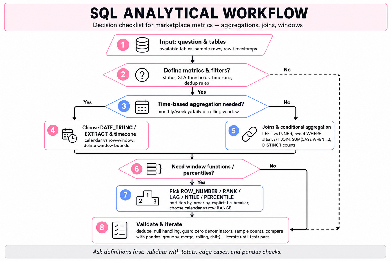
What's being tested

These questions test SQL analytical data manipulation for marketplace metrics: aggregating orders, joining customer/restaurant/event tables, grouping by time, ranking entities, and computing rates or percentiles. Interviewers are probing whether you can translate ambiguous DoorDash business definitions into correct SQL or Python logic with clean handling of timestamps, nulls, duplicates, and windowed metrics.

Patterns & templates

• Time-based aggregation — use `DATE_TRUNC`(`'month'`, `created_at`) or `EXTRACT` for monthly metrics; confirm timezone and order-status filters upfront.

• Conditional aggregation — compute rates with `SUM`(`CASE WHEN condition THEN 1 ELSE 0 END) * 1.0 / `COUNT`(*); guard against zero denominators.

• Entity ranking — use `ROW_NUMBER`, `RANK`, or `DENSE_RANK` with `PARTITION BY` for top customers, restaurants, or months; define tie-breaking explicitly.

• Windowed rolling metrics — use `AVG`, `SUM`, or `COUNT` over `ROWS BETWEEN` or date-range windows; distinguish row-count windows from calendar windows.

• Percentiles and quartiles — use `PERCENTILE_CONT`, `NTILE`(`4`), or `APPROX_PERCENTILE`; know whether the question needs exact thresholds or segmentation buckets.

• Event sequencing — use `LAG`, `LEAD`, and `ROW_NUMBER()` OVER (`PARTITION BY order_id ORDER BY event_ts`) to identify request flows and latest valid states.

• Python equivalent — map SQL patterns to `pandas`: `groupby`, `agg`, `merge`, `rank`, `rolling`, `quantile`, and `shift`; watch memory for large tables.

Common pitfalls

Pitfall: Counting rows instead of distinct orders or customers can inflate metrics after joins, especially with order-event or item-level tables.

Pitfall: Treating “late,” “cold,” or “completed” as obvious definitions without asking for SLA thresholds, cancellation handling, and timestamp source.

Pitfall: Using `WHERE` filters after a `LEFT JOIN` can silently turn it into an inner join and drop customers or restaurants with zero activity.