Truncated Normal And Probabilistic Sampling

What's being tested

These problems test whether you can define a truncated normal distribution, normalize its density correctly, and generate samples from it without introducing bias. The interviewer is probing your command of inverse-CDF sampling, rejection sampling, tail behavior, and the numerical tradeoffs among competing Monte Carlo methods. For a Data Scientist, this matters when modeling censored or constrained measurements, simulating counterfactuals, estimating uncertainty, or validating an estimator whose inputs are observed only within a range.

Core knowledge

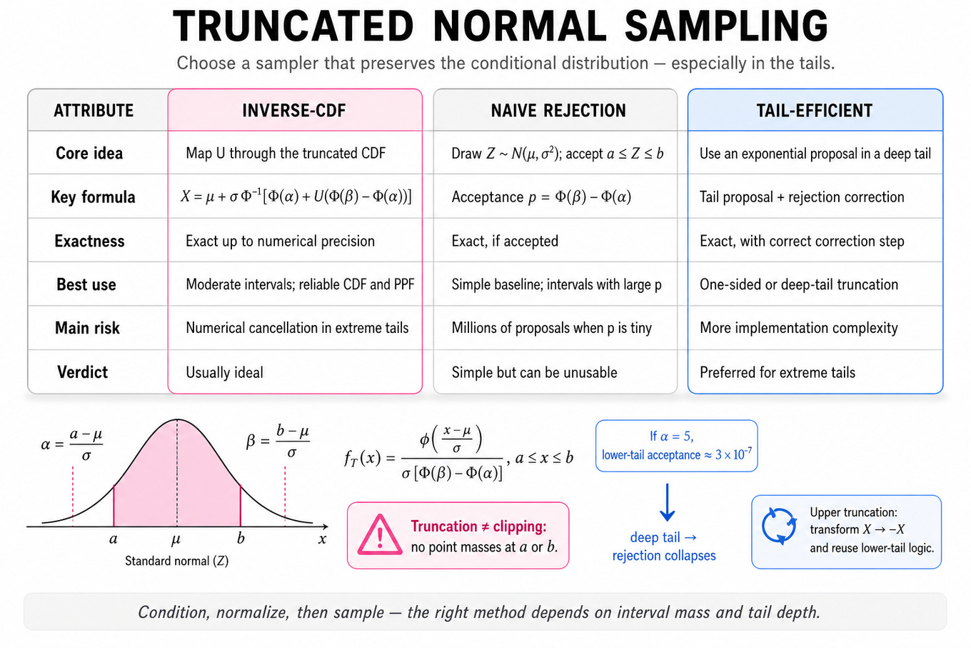
• A truncated normal is a normal random variable conditioned to lie in $[a,b]$: $X\sim N(\mu,\sigma^2)\mid a\le X\le b$. It is not the same as clipping values to the boundaries, which creates point masses at $a$ and $b$.

• Let $\alpha=(a-\mu)/\sigma$ and $\beta=(b-\mu)/\sigma$. The normalized density is $f_T(x)=\frac{\phi((x-\mu)/\sigma)}{\sigma[\Phi(\beta)-\Phi(\alpha)]},\qquad a\le x\le b,$ where $\phi$ and $\Phi$ are the standard normal PDF and CDF.

• Its CDF is

  {\Phi(\beta)-\Phi(\alpha)}.$$ This formula is the key to deriving both quantiles and **inverse-CDF sampling**; omitting the denominator incorrectly leaves the distribution unnormalized.

• Inverse-CDF sampling draws $U\sim\mathrm{Uniform}(0,1)$ and returns $X=\mu+\sigma\Phi^{-1}\left[\Phi(\alpha)+U\{\Phi(\beta)-\Phi(\alpha)\}\right].$ It is exact up to numerical precision and usually ideal for moderate intervals when reliable normal_cdf and normal_ppf implementations exist.

• Rejection sampling proposes $Z\sim N(\mu,\sigma^2)$ repeatedly and accepts it when $a\le Z\le b$. It is simple and exact, but its expected number of proposals is $1/p$, where $p=\Phi(\beta)-\Phi(\alpha)$. It becomes unusable when $p$ is extremely small.

• For one-sided lower truncation $X\ge a$, naive rejection has acceptance probability $1-\Phi(\alpha)$. If $\alpha=5$, this is roughly $3\times10^{-7}$, so millions of proposals may be needed per accepted draw.

Tip: Use a tail-efficient sampler, such as exponential rejection methods, for deep tails.

• For an upper truncation, transform signs: if $X\sim N(\mu,\sigma^2)$ conditioned on $X\le b$, then $-X$ is lower-truncated at $-\!b$ with mean $-\mu$. This reduces implementation complexity and helps reuse a well-tested lower-tail routine.

• Inverse-CDF calculations can lose precision when $\Phi(\alpha)$ is extremely close to $1$ or when $\Phi(\beta)-\Phi(\alpha)$ suffers catastrophic cancellation. Use stable survival-function APIs such as logsf, log-CDF arithmetic, or specialized truncated-normal libraries for extreme tails.

• The conditional mean is

  {\Phi(\beta)-\Phi(\alpha)}.$$ The conditional variance is $$\sigma^2\left[1+\frac{\alpha\phi(\alpha)-\beta\phi(\beta)} {\Phi(\beta)-\Phi(\alpha)} -\left(\frac{\phi(\alpha)-\phi(\beta)} {\Phi(\beta)-\Phi(\alpha)}\right)^2\right].$$ These are useful checks for simulations.

• Monte Carlo error decreases as $O(1/\sqrt n)$, not $O(1/n)$. To halve the standard error, you need approximately four times as many draws. Use independent random seeds, report uncertainty, and verify empirical moments or quantiles against theoretical values.

• Distinguish truncation from censoring and selection bias. Truncation removes observations outside a range; censoring records them only as “below” or “above” a threshold. Treating a censored sample as an ordinary truncated sample can bias parameter estimates and downstream experiment metrics.

Worked example: Define and sample a truncated normal

A strong candidate would first ask whether the interval is finite or one-sided, whether the goal is a mathematical derivation or production-quality sampling, and whether extreme-tail numerical stability matters. I would state that $X\sim N(\mu,\sigma^2)$ is conditioned on $a\le X\le b$, then organize the answer around the normalized PDF, the CDF, an exact sampling algorithm, and validation checks. I would derive the acceptance probability $p=\Phi(\beta)-\Phi(\alpha)$ before choosing between inverse-CDF and rejection sampling. The default implementation would use inverse-CDF sampling because it gives one accepted draw per uniform variate and avoids rejection inefficiency. I would explicitly flag the tradeoff that inverse-CDF is computationally predictable but can be numerically delicate in extreme tails, whereas rejection sampling is easier to explain but may be catastrophically slow there. I would validate simulated mean, variance, interval membership, and a histogram or probability integral transform against the theoretical distribution. I would also clarify whether parameters are known or estimated, because fitting a truncated likelihood requires including the same normalization constant. If I had more time, I would benchmark a tail sampler and test behavior across very narrow intervals and large standardized cutoffs.

A second angle: Generate Samples from Truncated Normal Distribution

For lower-tail truncation, the central issue shifts from deriving the bounded-interval formulas to algorithmic efficiency when $X\ge a$ and $a$ is many standard deviations above $\mu$. Inverse-CDF remains conceptually clean, but evaluating $1-\Phi(\alpha)$ directly may underflow or lose precision. A strong answer compares naive rejection with exponential-envelope or specialized normal-tail samplers and quantifies acceptance rather than merely naming methods. The practical choice depends on the tail threshold, sample volume, and whether the environment provides stable logsf and ppf functions.

Common pitfalls

Pitfall: Saying “sample a normal and clip values outside the interval” is wrong because clipping creates boundary point masses and does not produce the conditional distribution. State clearly that rejected values must be resampled, or use the inverse conditional CDF.

A tempting answer gives the correct PDF but forgets the normalization term $\Phi(\beta)-\Phi(\alpha)$. That density integrates to the probability of landing in the interval, not to one; explicitly checking the integral and conditional CDF prevents this analytical mistake.

Another weak response lists inverse-CDF and rejection sampling without discussing numerical stability or acceptance rate. A better Data Scientist answer quantifies $1/p$, identifies extreme-tail failure modes, and explains how empirical moments or quantiles would validate the implementation.

Connections

An interviewer may pivot to maximum likelihood under truncation, censored-data models such as Tobit regression, or importance sampling for rare events. They may also connect this to confidence intervals, Bayesian posterior sampling, variance reduction, and the distinction between selection effects and genuine population differences.

Further reading

• Robert, “Simulation of truncated normal variables” — classic methods for efficient simulation, especially in tail regions.

• Robert and Casella, Monte Carlo Statistical Methods — rigorous treatment of rejection sampling, importance sampling, and Monte Carlo error.

• Nadarajah, “Some truncated distributions” — broader formulas and properties for truncated distributions.