Apache Spark Interview Questions for Data Engineers: Shuffles, Partitions, and Debugging

A useful Apache Spark interview answer explains where the work happens, which evidence identifies the bottleneck, and how a proposed fix preserves the result. “Increase the partitions” is incomplete until you can say which partitions, why their current size is a problem, and what you expect to change.

This guide covers batch DataFrame and SQL execution, with RDD concepts where they clarify the mechanism. Engine behavior is grounded in Apache Spark 4.0.1 documentation. That is a versioned reference baseline, not a claim that every employer uses that release. Examples and diagnostic scenarios are original preparation exercises, not production benchmarks or guaranteed interview questions.

Start with PracHub's Explain Spark Execution and Optimization, then use the questions below to practice moving from a definition to a diagnosis.

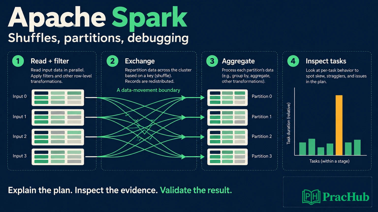
Conceptual Spark flow from reading and filtering through an exchange, aggregation, and inspection of task metrics

What is a shuffle, and why does it create a bottleneck?

Official mechanism: a shuffle redistributes data so records needed together can be processed together. It can involve serialization, network transfer, disk I/O, and sorting. The RDD programming guide explains shuffle operations and their costs. Local transformations such as a simple filter do not inherently require that redistribution.

For an aggregation by customer, rows for the same customer must contribute to the same final result. Spark can perform partial aggregation before the exchange, reducing the amount transferred. Do not assume that every input row crosses the network unchanged, or that every join must shuffle both sides.

In a stage, tasks process partitions of the stage's work. Shuffle dependencies separate stages; executors run tasks scheduled by the driver. SQL execution can produce multiple jobs, including work for adaptive execution, so avoid insisting that one action always corresponds to exactly one job.

Practice answer: “I would inspect the physical plan to locate the exchange, then check how much data its tasks write and read. I would reduce unnecessary input before changing cluster size.” That connects the mechanism to an observable next step.

What should you look for in an execution plan?

Use DataFrame.explain to inspect a plan. explain("formatted") presents a physical-plan outline and operator details; explain("cost") includes logical-plan statistics when available. Treat those statistics as inputs to a hypothesis, not measured runtime evidence.

For a simple read-filter-aggregate pipeline, identify the scan, filters, partial aggregation, exchange, and final aggregation. Then ask whether a filter can be pushed into the source and whether unnecessary columns survive into an expensive operator.

If the physical plan contains an unexpected join or exchange, trace it back to the expression that required it. A convenient helper function can hide a repartition or a wide transformation. Read the plan produced by the actual query, rather than predicting execution from the number of lines of PySpark.

After execution, inspect the final adaptive plan where available. A pre-execution plan and the plan used after runtime statistics arrive need not be identical. Explain any change before comparing two runs.

Which kind of partition are you changing?

The word “partition” can describe several different boundaries. Naming the boundary prevents configuration changes that have no effect on the slow stage.

Partition boundary	The question to ask
Storage layout, such as date directories	Can the read avoid irrelevant data?
Input scan work	How are files or source splits assigned to tasks?
Shuffle output	How much work reaches each downstream partition?
Final write work	What parallelism and file layout does the sink need?

The SQL tuning reference documents spark.sql.shuffle.partitions, whose upstream default is 200, and file-source controls such as spark.sql.files.maxPartitionBytes. They govern different parts of execution. Neither gives you a universal partition count for a dataset.

Original sizing exercise: suppose a stage writes 64 GiB of shuffle data. Dividing by an illustrative 128 MiB target suggests 512 partitions before considering skew, adaptive coalescing, and task overhead. This is a starting estimate, not a prescription: shuffle bytes are not the same as the in-memory working set.

Ask what changed when data volume grew. If average partition size doubled and most tasks now spill, more downstream parallelism may help. If one key dominates one partition, increasing the count alone may leave that key concentrated in a single destination.

When should you use repartition instead of coalesce?

Official API behavior: repartition changes partitioning and can distribute rows by specified expressions. With partitioning columns, the resulting DataFrame is hash-partitioned. It is useful when redistribution is needed, but that work has a cost.

Coalesce reduces partitions through a narrow dependency without adding a shuffle. The documentation warns that a drastic reduction can concentrate computation on fewer nodes. Asking for more partitions through coalesce does not provide the redistribution that repartition does.

In an interview, distinguish reducing tiny output tasks from fixing an unbalanced distribution. coalesce(1) may produce a convenient small export, but it can become a severe bottleneck for a large result. “One output file” is a delivery requirement to examine, not an automatic performance improvement.

Also distinguish partition count from file count. A partitioned write, a file-size control, or sink behavior can affect the number of files produced. Verify the observed output instead of promising that a given partition count always means exactly that many files.

Is the slow stage skewed, or is every task overloaded?

The Spark Web UI guide describes stage and task metrics, including duration, shuffle activity, spill, and executor information. Compare distributions rather than relying on one total or average.

Original diagnostic comparison: in Case A, most tasks read roughly 600 MiB, take similar times, and spill heavily. In Case B, most tasks read about 40 MiB and finish quickly, while one reads 8 GiB and runs much longer. The symptoms suggest different investigations; neither is a complete diagnosis by itself.

For Case A, inspect the working set, concurrent tasks per executor, and whether unnecessary rows or columns reached the stage. For Case B, inspect key frequencies, join multiplicity, and whether the outlier repeatedly handles the same data. More executors can leave a single oversized task unchanged.

Compare the same partition across task attempts. If failures follow one data slice across machines, suspect a data-dependent problem. If unrelated tasks fail on one executor, investigate that executor's logs and resource condition. A long task with ordinary input size may instead involve slow I/O, expensive code, or a problematic machine.

State the observation that would change your mind. “If the outlier has normal shuffle input but excessive garbage collection, I would investigate memory behavior rather than assuming key skew.” This makes your reasoning testable.

How do join choice and AQE change the investigation?

Official behavior: the SQL performance-tuning guide describes broadcast joins and Adaptive Query Execution. AQE uses runtime statistics and can coalesce post-shuffle partitions, change eligible join strategies, and optimize supported skewed joins. It is enabled by default upstream in this reference version, but session settings and platform defaults must still be checked.

Broadcasting a suitable small side can avoid shuffling the large side. Judge size from the actual projected data and memory needs, not only row count. AQE is not a guarantee that every hot aggregation key or unsuitable broadcast will repair itself.

Correctness check before tuning: a join can become huge because the key is not unique. If one key has three rows on the left and four on the right, an inner equijoin produces twelve matching rows for that key. That may be correct many-to-many behavior or an unintended change of grain.

Inspect counts and uniqueness before salting or adding memory. If the requirement is one current record per key, define a deterministic rule for selecting it. Arbitrary deduplication can make a job faster while changing its answer.

How can salting produce the wrong average?

Original exercise: salting splits a hot key into subkeys so partial work can be distributed, followed by recombination. The recombination must preserve the aggregate's meaning.

Suppose one salt bucket contains 10, 10, 10 and another contains 20. Their means are 10 and 20. Averaging those means gives 15, but the original four values average to 12.5.

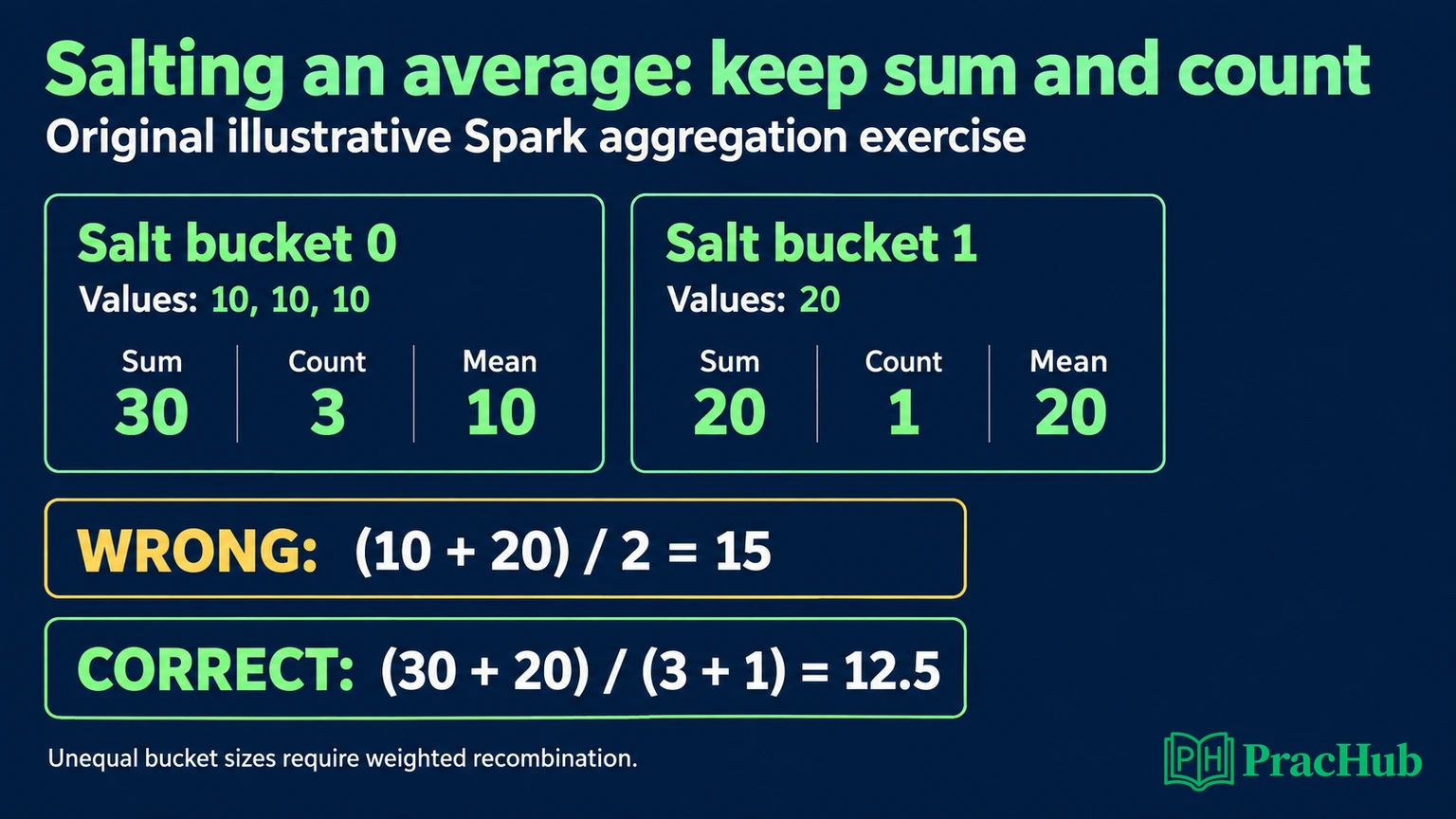
Salted-average example showing why partial sums and counts must be recombined instead of averaging unequal-sized bucket means

Carry each bucket's sum and count instead. Combine sums and counts, then divide once:

partials = [(30, 3), (20, 1)]  # (sum, count)
total_sum = sum(s for s, n in partials)
total_count = sum(n for s, n in partials)
mean = total_sum / total_count
assert mean == 12.5

This Python fixture demonstrates the algebra; it is not a distributed Spark benchmark. In a Spark implementation, the first aggregation groups by the original key plus salt, and the second removes the salt while merging sufficient statistics. For averages that ignore null values, carry the count of contributing values rather than all rows, and define the all-null result.

Spark already handles the semantics of its built-in average; this counterexample concerns a manual rewrite. Salting is not the default fix for every aggregation. Measure the remaining bottleneck before adding another grouping step.

Do not generalize this recipe to every aggregate. Exact distinct counts cannot be combined by simply adding per-bucket distinct counts when values overlap. A median requires more information than partial sums and counts. Before recommending salting, explain both the distribution benefit and the proof that recombination preserves the answer.

When does caching help, and when does it hurt?

The DataFrame.persist documentation describes persisting a DataFrame after it is first computed so subsequent operations can reuse it. Calling persist does not eagerly calculate every partition by itself.

Preparation recommendation: identify an expensive intermediate result that multiple actions reuse. Compare the cost of computing and storing it with the saved recomputation. Caching a one-use result may add overhead and memory pressure without a useful return.

Measure both the first run and subsequent runs, and keep cache state explicit in comparisons. Otherwise an apparent optimization may just compare a cold execution with a warm one. Release persisted data when it is no longer needed.

Caching also does not correct a bad join grain, an oversized result collected to the driver, or invalid aggregation logic. Fix the relevant contract before preserving its output more efficiently.

How do you debug a failed stage?

Start with the earliest useful failure evidence, not just the final “job aborted” message. Record the application, stage, task attempt, executor, exception, and input involved. Preserve the code version and configuration so the failure can be compared with a successful run.

Recommended triage: separate a deterministic parsing error from an executor memory failure or an inability to fetch shuffle output. A fetch failure identifies unavailable shuffle data; investigate upstream executor loss, storage, and network evidence before treating a larger timeout as a fix.

The monitoring guide explains event logging and the History Server. Enable event logging before the application runs if you need to inspect its UI after termination. A completed application's history is valuable when the failure is intermittent or the original driver is gone.

Finally, examine sink behavior under retries. Recovering a task does not, by itself, prove that an external side effect occurs only once. Validate row counts, key uniqueness, aggregate reconciliation, and rerun behavior alongside duration and resource use.

Five questions to rehearse with PracHub

These are candidate-reported practice records across employers. Use official documentation to check Spark behavior; the records are not a promise of your next interview. Some solution details may require access.

PracHub question	Follow-up to rehearse
Explain Spark Execution and Optimization	Locate the exchange and explain its task-level evidence
Design MapReduce and Spark jobs	Explain which partial results can safely be combined
Reason About Duplicate Data and Scaling in Spark	Preserve key semantics while changing execution
Data Pipeline Reliability, Backfills, and Spark Optimization	Distinguish skew from broad resource pressure
Optimize MapReduce performance	Separate network volume, task balance, and local computation

Close a practice answer with the metric you expect to improve and the invariant that must remain unchanged. Start with Design MapReduce and Spark jobs, then use the salted-average counterexample to test whether your proposed aggregation is valid.

For Delta Lake, governance, and broader platform questions, continue with the Databricks data engineer guide.

Sources and Further Reading

Research checked September 8, 2026. Configuration and behavior use the versioned 4.0.1 references above; verify your deployed runtime. Example sizes, timings, and values are illustrative.