SQL Retention Interview Questions: Cohort Definitions, Incomplete Windows, and Correct Denominators
Quick Overview
Define the cohort and observation cutoff, then verify exact-day and on-or-after retention using one complete original dataset.
SQL retention interview questions become easier when you decide who belongs in the denominator before joining activity. A query can execute successfully and still turn new users into apparent churn, count one enthusiastic user twice, or answer a different retention question from the one you were asked.
Start with PracHub's D7 retention SQL exercise, then use the complete dataset below to inspect the boundary cases. The goal is to explain every counted user, not merely produce a plausible percentage.
Evidence boundary: Official documentation supports the metric distinctions and SQLite behavior cited here. The dataset, queries, expected outputs, and interview advice are original PracHub practice. They are not a company's assessment or a candidate report.

What exactly does “D7 retention” mean?
Before writing SQL, define the start event, return event, identity, time convention, and observation cutoff. “People who signed up and came back” leaves several different calculations possible. Ask one concrete clarifying question for each ambiguity that changes a result.
Official metric context: Amplitude distinguishes Return On, which requires activity on the specified day, from Return On or After, which accepts activity on that day or later. Its overall calculations exclude incomplete retention intervals. These are documented product definitions, not proof that every interview uses the same convention. Amplitude retention calculations
For this exercise, cohort entry is the user's recorded signup date. A return is an active event; an email event does not count. Identity is user_id. D7 is the seventh UTC calendar date after signup, and the dataset is complete through the end of August 10, 2026.
An August 1 signup therefore reaches D7 on August 8. We are not asking whether the user returned during the first seven days, nor whether exactly 168 hours elapsed. With timestamped data, a late-night signup and an early-morning return can expose that distinction immediately.
We calculate two outcomes: activity exactly on D7, and activity on or after D7 observed by the fixed cutoff. The second outcome gives older cohorts more opportunity to return. It must be labeled with that observation boundary rather than presented as a finalized lifetime probability.
Load the complete twelve-user dataset
The following setup is the entire original fixture. Run it in an empty SQLite database. There are twelve signup records and twelve event rows. Some users have no events, one event is duplicated, and one lies beyond the reporting cutoff.
CREATE TABLE users(user_id INTEGER PRIMARY KEY, signup_day TEXT NOT NULL);
CREATE TABLE events(user_id INTEGER, event_day TEXT, event_type TEXT);
INSERT INTO users VALUES
(1,'2026-08-01'),(2,'2026-08-01'),(3,'2026-08-01'),
(4,'2026-08-01'),(5,'2026-08-02'),(6,'2026-08-02'),
(7,'2026-08-02'),(8,'2026-08-02'),(9,'2026-08-04'),
(10,'2026-08-04'),(11,'2026-08-08'),(12,'2026-08-08');
INSERT INTO events VALUES
(1,'2026-08-08','active'),(1,'2026-08-08','active'),
(2,'2026-08-09','active'),(3,'2026-08-07','active'),
(4,'2026-08-08','email'),(5,'2026-08-09','active'),
(6,'2026-08-10','active'),(7,'2026-08-09','active'),
(7,'2026-08-10','active'),(9,'2026-08-10','active'),
(10,'2026-08-11','active'),(11,'2026-08-09','active');
The date strings are already normalized UTC reporting dates. Engine behavior: SQLite's date() accepts supported date representations and modifiers such as '+7 days', returning a date string. This example avoids implicit machine-local timezone conversion. SQLite date functions
In a production dataset, a signup table might contain retries, multiple accounts, imports, or historical corrections. The primary key here deliberately removes those ambiguities. If your real source is an event log, establish a canonical first signup before counting cohort users; taking the minimum date only inside a recent extraction can misclassify older users as new.
The August 11 event for user 10 is included to test the cutoff. Its presence in the physical table does not authorize using it in an August 10 report. A reproducible historical query must honor the declared reporting boundary even when the warehouse contains newer rows.
Derive one record per user before aggregating
Build a small intermediate relation containing cohort date, D7 date, eligibility, and two return flags. It gives you a place to inspect the calculation before grouping away the evidence.
CREATE TEMP VIEW user_flags AS
SELECT u.user_id, u.signup_day,
  date(u.signup_day, '+7 days') AS d7,
  CASE WHEN date(u.signup_day, '+7 days')
    <= '2026-08-10' THEN 1 ELSE 0 END AS eligible,
  MAX(CASE WHEN e.event_day =
    date(u.signup_day, '+7 days') THEN 1 ELSE 0 END) AS exact_d7,
  MAX(CASE WHEN e.event_day >=
    date(u.signup_day, '+7 days') THEN 1 ELSE 0 END) AS d7_plus
FROM users u
LEFT JOIN events e ON e.user_id = u.user_id
  AND e.event_type = 'active'
  AND e.event_day <= '2026-08-10'
GROUP BY u.user_id, u.signup_day;
The LEFT JOIN preserves users with no qualifying return. Event-type and cutoff conditions belong in its ON clause here. Moving them into a WHERE condition on the event columns would discard unmatched users, silently shrinking the denominator.
Each return flag uses a maximum over zero-or-one values, so two qualifying events still contribute one user. Engine behavior: SQLite's aggregate functions operate over each group; COUNT(*) counts rows, while COUNT(column) ignores NULL values. Choose the expression that matches the intended grain. SQLite aggregate functions
Eligibility is independent of activity. User 8 is eligible despite having no events. User 11 is ineligible despite having an observed active event. “Has an event” and “has had a complete opportunity to return on D7” are different tests.
The raw flags for an ineligible user should not be displayed as a settled outcome. Keep eligibility alongside them, or expose NULL in your reporting view. That prevents a dashboard consumer from interpreting an unfinished window as an observed failure.
Check the answer user by user
This ledger is the expected result before any percentages. A dash means the D7 outcome is not yet observable under this report's contract; it does not mean the user failed to return.
| User | Eligible for D7? | Exact D7 | Observed D7 or later |
|---|---|---|---|
| 1 | Yes | 1 | 1 |
| 2 | Yes | 0 | 1 |
| 3 | Yes | 0 | 0 |
| 4 | Yes | 0 | 0 |
| 5 | Yes | 1 | 1 |
| 6 | Yes | 0 | 1 |
| 7 | Yes | 1 | 1 |
| 8 | Yes | 0 | 0 |
| 9 | No | — | — |
| 10 | No | — | — |
| 11 | No | — | — |
| 12 | No | — | — |
User 1's duplicate event does not add another person. User 2 returns on D8, so qualifies only for the later-return definition. User 3 returns on D6, which qualifies for neither measure. User 4 has an email event on D7, but no qualifying activity.
User 7 has activity on D7 and D8 and still counts once in each relevant numerator. User 8 remains a non-returning member of the mature cohort. Users 9–12 have not reached D7 by August 10, including user 10 whose future row must be excluded.
This ledger is also a debugging tool. If a query disagrees, identify the first user whose classification differs. Inspect that user's signup date and events before rewriting the aggregate. A percentage alone cannot reveal whether the mistake came from dates, duplication, event semantics, or eligibility.
Calculate cohort rates without turning NULL into zero
Aggregate the intermediate records, keeping total cohort size separate from the number eligible for this interval:
SELECT signup_day, COUNT(*) AS cohort_users,
  SUM(eligible) AS eligible_users,
  SUM(eligible * exact_d7) AS exact_users,
  ROUND(1.0 * SUM(eligible * exact_d7)
    / NULLIF(SUM(eligible), 0), 3) AS exact_rate,
  SUM(eligible * d7_plus) AS plus_users,
  ROUND(1.0 * SUM(eligible * d7_plus)
    / NULLIF(SUM(eligible), 0), 3) AS plus_rate
FROM user_flags GROUP BY signup_day ORDER BY signup_day;
The expected output is shown below. Dates are in August 2026; All is cohort size, N is eligible users, and each outcome cell shows users / rate.
| Date | All | N | D7 | D7+ |
|---|---|---|---|---|
| 08-01 | 4 | 4 | 1 / 0.250 | 2 / 0.500 |
| 08-02 | 4 | 4 | 2 / 0.500 | 3 / 0.750 |
| 08-04 | 2 | 0 | 0 / NULL | 0 / NULL |
| 08-08 | 2 | 0 | 0 / NULL | 0 / NULL |
The zero numerators in the last two rows are counts of eligible returners, not proof of zero retention. With no eligible denominator, the rate is NULL. A presentation layer can display “not yet observable” instead of a blank, but should not replace it with 0%.
The 1.0 explicitly produces a fractional result. NULLIF protects the zero-denominator case, and rounding happens only for display. Preserve sufficient precision upstream so a rounded dashboard value does not become the input to another calculation.
Pool mature users and expose the wrong denominator
For the overall result, sum eligible people and returning people across cohorts. Do not average displayed percentages without considering cohort sizes.
SELECT SUM(eligible) AS eligible_users,
  SUM(eligible * exact_d7) AS exact_users,
  1.0 * SUM(eligible * exact_d7) / SUM(eligible) AS exact_rate,
  SUM(eligible * d7_plus) AS plus_users,
  1.0 * SUM(eligible * d7_plus) / SUM(eligible) AS plus_rate
FROM user_flags;
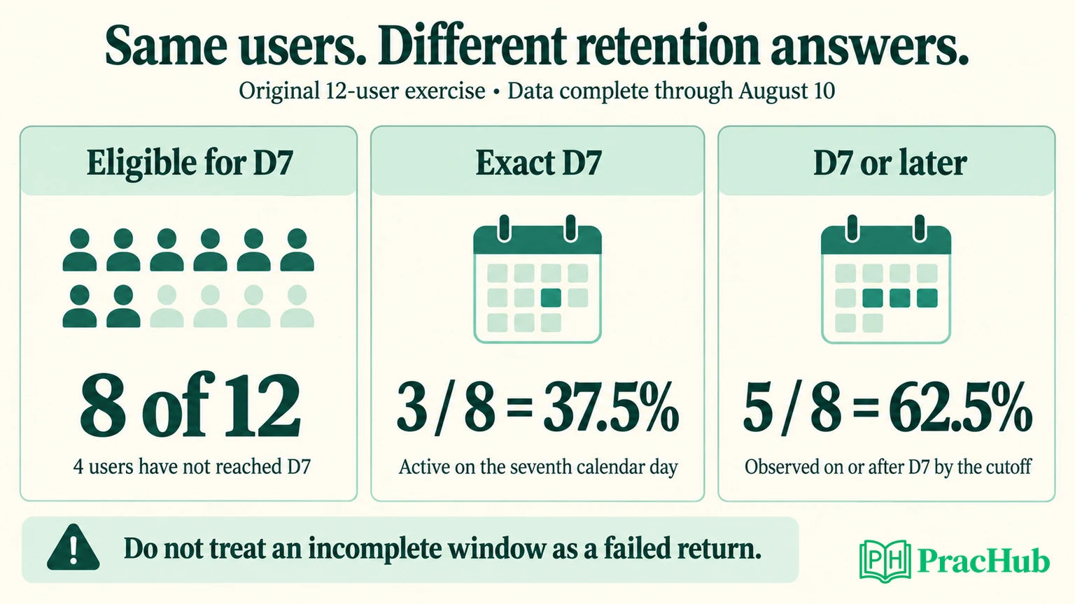
Executed original result: Eight users are eligible. Three return exactly on D7, giving 37.5%. Five return on D7 or later by August 10, giving 62.5%. The SQL outputs, cohort rows, and twelve user classifications were checked against explicit expected values.
Dividing the exact-day numerator by all twelve signups instead gives 25%. That number treats four unfinished windows as failures. It answers neither the mature-cohort D7 question nor a defensible estimate of those new users' eventual behavior.
Averaging the two mature cohort rates happens to work here because both cohorts contain four users. That is a property of this fixture, not a general aggregation rule. If one cohort had forty users and the other four, an unweighted average would give each cohort equal influence despite very different population sizes.
Explain what changes when the window changes
An interviewer may ask for a fairer comparison between cohorts of different ages. One option is a bounded return interval, such as activity from D7 through D14, using only cohorts whose D14 has fully elapsed. That changes both the event predicate and eligibility threshold; editing only the numerator is incomplete.
Do not label our current D7-or-later result as D7–D14 retention. August 1 users have only been observed through D9, while August 2 users have reached D8. The fixed reporting date makes the computation reproducible, but does not equalize follow-up opportunity.
If the cutoff moves forward, exact-D7 classifications for already complete cohorts should remain stable when the underlying records are unchanged. The observed on-or-after numerator may increase as later returns arrive. Previously immature users can also enter the denominator, so the pooled rate need not move in only one direction.
Late-arriving records require another distinction: event time determines the retention day, while ingestion time determines what the report knew when it ran. A corrected historical report and a faithful “as known then” report can legitimately differ. State which one the interview asks you to produce.
Use boundary checks before optimizing
Rehearse the failure cases deliberately. Remove the duplicate event and confirm unchanged rates. Move a qualifying event from D7 to D6 and confirm its exact-day flag changes. Replace active with email and ensure it no longer counts. Keep an inactive eligible user in the denominator.
Also test the first eligible date and the first ineligible date around the cutoff. If today is only partly ingested, “through today” is not a complete calendar-day boundary. Use the last complete reporting date or explicitly model partial observation.
For larger datasets, reduce qualifying events to the needed user-day grain, restrict scans to relevant dates, and examine the query plan. Those changes should preserve the user ledger and aggregate answers. Faster SQL with a different denominator is a different metric, not a successful optimization.
Five questions for transferring the method
These linked records provide related practice across companies. They are not claims that every employer asks this exact fixture.
| PracHub question | What to verify |
|---|---|
| Write SQL window functions for D7 retention | Define the date boundary before choosing a window function. |
| Compute 30-day power users and 7-day retention | Keep activity qualification separate from retention eligibility. |
| Compute signup rate and retention from raw logs | Establish identity and cohort entry before aggregating logs. |
| Aggregate D1 retention cohorts in SQL | Transfer the same reasoning to a different interval. |
| Design KPI dashboard tables: retention, weekly rollups, timezone | Preserve grain and timezone semantics in derived tables. |
Return to the D7 SQL question and state your denominator aloud before writing the final aggregate. Your explanation should identify who is counted, who is not yet observable, and which event would change each user's result.
Sources and Further Reading
- Amplitude retention calculations — documented Return On and Return On or After definitions.
- SQLite date and time functions — supported dates, modifiers, and UTC behavior.
- SQLite aggregate functions — grouped counting and aggregation semantics.
Sources checked September 9, 2026. All example data and expected outputs are original practice material.
Comments (0)