Causal Inference And Identification

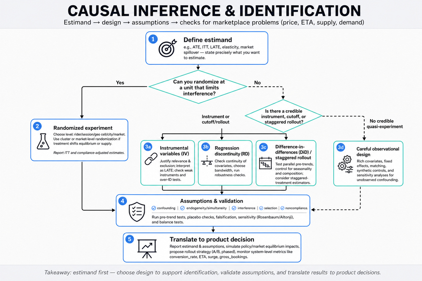
What's being tested

Interviewers are probing whether you can separate correlation from causation in Uber-style marketplace problems where price, ETA, demand, and supply move together. A strong Data Scientist must define the right estimand, choose an identification strategy, defend assumptions, and translate the result into a product or marketplace decision. Uber cares because metrics like conversion_rate, ETA, surge_multiplier, gross_bookings, and driver utilization are jointly determined; naive regressions can confidently recommend the wrong lever. Expect pressure on endogeneity, selection bias, interference, noncompliance, and whether your proposed estimate would actually answer the business question.

Core knowledge

• Estimand first, method second. State whether you want the average treatment effect: $ATE = E[Y(1)-Y(0)]$, intent-to-treat effect, local average treatment effect, elasticity, or market-level spillover effect. For Uber, “effect of ETA on conversion” differs from “effect of showing a lower ETA prediction.”

• Confounding occurs when treatment assignment is related to potential outcomes. Example: shorter ETA often occurs in dense areas with higher baseline conversion, so regressing conversion_rate on ETA overstates the causal benefit of reducing ETA unless geography, time, demand, rider intent, and supply are handled.

• Endogeneity and simultaneity are central in price–ETA trade-offs. Price affects demand, demand affects driver availability, driver availability affects ETA, and ETA affects conversion. A naive model like $Conversion_i = \beta_0 + \beta_1 Price_i + \beta_2 ETA_i + \epsilon_i$ usually violates $E[X_i\epsilon_i]=0$.

• Randomized experiments are the cleanest design when feasible. Randomize at the unit where interference is limited: rider, session, geo cell, city, or time block. If treatment can affect marketplace equilibrium, rider-level randomization may contaminate control via shared driver supply, so cluster or market-level randomization may be needed.

• Difference-in-differences estimates treatment effects by comparing treated and control changes over time:
  $\hat{\tau}_{DiD}=(\bar{Y}_{T,post}-\bar{Y}_{T,pre})-(\bar{Y}_{C,post}-\bar{Y}_{C,pre})$
  The key assumption is parallel trends, not equal levels. Always check pre-trends, seasonality, rollout timing, and compositional shifts.

• Instrumental variables handle unobserved confounding when you have a source of exogenous variation. A valid instrument $Z$ must satisfy relevance, $Cov(Z,X)\neq0$, exclusion, $Z$ affects $Y$ only through $X$, and independence from unobserved outcome drivers. In Uber contexts, candidates might discuss weather shocks, randomized price nudges, supply-side constraints, or dispatch rule variation, but must defend exclusions carefully.

• Two-stage least squares estimates causal effects using predicted treatment variation. First stage: $X_i=\pi_0+\pi_1Z_i+\gamma W_i+u_i$. Second stage: $Y_i=\beta_0+\beta_1\hat{X}_i+\delta W_i+\epsilon_i$. Report first-stage strength, often using an F-statistic rule of thumb above 10, and interpret $\beta_1$ as a LATE for compliers.

• Elasticity estimation often uses log-log models: $\log(Q_i)=\alpha+\beta\log(P_i)+\gamma W_i+\epsilon_i$, where $\beta$ is price elasticity. But if price is dynamically set based on demand, the model identifies association unless price variation is randomized or instrumented.

• Interference violates SUTVA when one user’s treatment affects another user’s outcome. In rideshare, changing ETAs or prices for some riders changes driver availability, wait times, and conversion for others. Handle with cluster randomization, exposure mappings, market-level aggregates, or estimands like direct effect, spillover effect, and total effect.

• Noncompliance means assignment differs from actual exposure. For example, a rider assigned to see a new ETA treatment may not open the app, or a city assigned to a pricing change may only partially roll it out. Estimate ITT for policy impact; use IV/Wald estimators for complier effects: $\frac{E[Y|Z=1]-E[Y|Z=0]}{E[D|Z=1]-E[D|Z=0]}$.

• Diagnostics matter as much as estimation. For experiments, check balance, sample ratio mismatch, guardrail metrics, and heterogeneous treatment effects. For DiD, inspect pre-period event-study coefficients. For IV, test instrument strength and argue exclusion qualitatively; no statistical test can fully prove exclusion.

• Aggregation level changes interpretation. Session-level data supports individual conversion models, while geo-hour or city-week panels capture marketplace equilibrium. With millions of sessions, standard errors can still be wrong if treatment varies by market; use cluster-robust standard errors at the assignment or shock level, not just row-level n.

Worked example

For “Estimate price–ETA trade-offs causally”, a strong candidate would start by clarifying the decision: are we estimating how much conversion changes if Uber increases price holding ETA fixed, decreases ETA holding price fixed, or changes a dispatch/pricing policy that moves both? They would define the outcome, likely conversion_rate, completed_trips, or contribution margin, and specify whether the unit is request, session, geo-hour, or market-day. The answer should be organized around four pillars: first, explain why naive regression is biased because price, ETA, demand, and supply are jointly determined; second, propose a preferred experiment if feasible, such as randomized price or ETA-display perturbations with guardrails; third, offer an observational fallback using IV or DiD; fourth, discuss diagnostics and interpretation.

A candidate might propose an IV where random price nudges or algorithmic threshold discontinuities shift price but are plausibly unrelated to rider intent except through price. They should immediately flag the exclusion restriction: if the same mechanism also changes ETA, the instrument may not isolate price unless ETA is modeled as a separate endogenous variable or the estimand is the joint policy effect. The 2SLS skeleton would use first-stage models for price and/or ETA, then a second-stage conversion model with market-time controls and clustered standard errors. A key tradeoff is between internal validity and external validity: a small randomized nudge gives clean identification around current prices but may not extrapolate to large surge changes. To close, they could say: “If I had more time, I’d estimate heterogeneous elasticities by city, rider segment, and trip purpose, and compare short-run conversion effects with marketplace equilibrium effects on driver supply.”

A second angle

For “Evaluate ETA Impact on Conversion”, the same causal logic applies, but the treatment is more likely a service quality variable than a direct product knob. The tempting analysis is to bucket sessions by observed ETA and compare conversion, but that confounds ETA with density, weather, airport trips, rider urgency, and driver supply. A stronger framing distinguishes the effect of actual ETA reduction from the effect of displaying a different ETA prediction. If experimenting on actual ETA is hard because dispatch changes affect the whole market, the candidate should discuss cluster randomization or quasi-experimental variation in supply shocks. The best answer also notes interference: reducing ETA for treated riders may increase ETA for untreated riders competing for the same drivers.

Common pitfalls

Pitfall: Treating controls as a cure-all.

A common analytical mistake is saying “I’ll control for city, time, and rider features, then regress conversion on ETA.” That may reduce observed confounding, but it does not solve unobserved intent, simultaneity, or marketplace equilibrium effects. A better answer explicitly states the identifying assumption and why it may or may not be believable.

Pitfall: Not naming the estimand.

Candidates often jump into 2SLS, DiD, or experimentation without saying what effect they want. Interviewers will push: is this the effect on riders exposed to treatment, all riders in the market, complisers, or the total marketplace effect including spillovers? Start with the estimand, then choose the design.

Pitfall: Ignoring interference in a two-sided marketplace.

A rider-level A/B test sounds clean but can fail when treated and control users share the same driver pool. If the treatment changes driver allocation, wait times, or surge, control outcomes are contaminated. A stronger answer proposes geo-level randomization, switchback experiments, or explicit spillover estimands.

Connections

Interviewers may pivot from causal identification into experiment design, especially switchback tests, cluster randomization, power, and guardrail metrics. They may also connect to metric design, marketplace dynamics, ranking/model evaluation, or segmentation, asking whether the estimated effect differs by city, time of day, rider tenure, or supply conditions.

Further reading

• Mostly Harmless Econometrics — practical treatment of IV, DiD, regression, and identification assumptions.

• Causal Inference: The Mixtape — accessible examples of DiD, IV, event studies, and modern applied causal inference.

• Design and Analysis of Switchback Experiments — useful for marketplace experiments where interference makes user-level randomization problematic.