Causal Inference, Confounding, And Matching

What's being tested

Interviewers are probing whether you can separate causal impact from correlation when product behavior changes outside a clean randomized experiment. For a LinkedIn Data Scientist, this matters because product decisions often depend on metrics like job_applications, apply_start_rate, notification_ctr, profile_views, or sessions_per_member, where user mix, market conditions, ranking changes, and seasonality can all confound the observed trend. You are expected to reason through confounding, selection bias, heterogeneous treatment effects, and Simpson’s paradox, then propose an analysis that estimates the right causal quantity. Strong answers define the estimand, diagnose bias, segment intelligently, and communicate uncertainty rather than overclaiming.

Core knowledge

• Causal inference starts with an estimand: what effect are we trying to estimate, for whom, over what time window? Common estimands include ATE $E[Y(1)-Y(0)]$, ATT $E[Y(1)-Y(0)\mid T=1]$, and segment-specific effects such as impact on new job seekers in US metro areas.

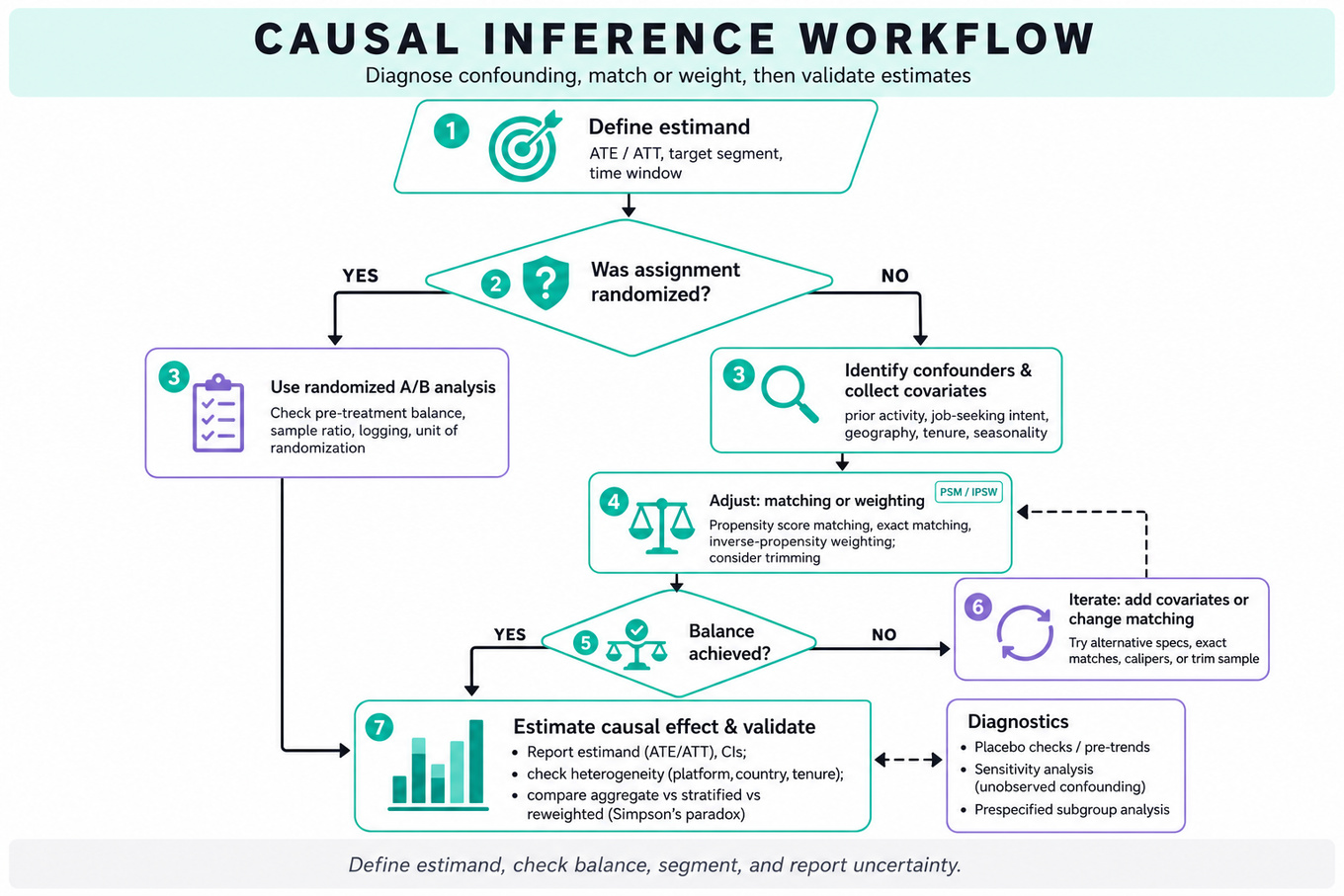
• Confounding occurs when a variable affects both treatment assignment and outcome. If active job seekers are more likely to receive an email and also more likely to apply, raw email recipients versus non-recipients will overstate impact unless you adjust for prior activity, job-seeking intent, geography, seniority, and seasonality.

• Randomized A/B tests solve confounding in expectation because treatment assignment is independent of potential outcomes: $T \perp (Y(0),Y(1))$. Still, you must check sample ratio mismatch, pre-treatment balance, logging gaps, interference between users, novelty effects, and whether the randomization unit matches the metric unit.

• Simpson’s paradox happens when aggregate results reverse after conditioning on a key variable. For example, a redesign may look negative overall but positive in every city if traffic shifted toward cities with lower baseline application rates. Always compare aggregate, stratified, and reweighted estimates.

• Heterogeneous treatment effects are expected in marketplace products. A job-application redesign may help mobile users but hurt desktop users, or help entry-level seekers but hurt senior roles. Pre-specify critical cuts like country, platform, member tenure, job-seeker intent, and recruiter/job supply density to avoid cherry-picking.

• Propensity score matching estimates $e(X)=P(T=1\mid X)$ using pre-treatment covariates, often via logistic regression, XGBoost, or generalized boosted models. Match treated and control users with similar $e(X)$, then estimate outcomes within the matched sample. The key assumption is conditional ignorability: $(Y(0),Y(1)) \perp T \mid X$.

• Common support is mandatory for matching. If redesigned users have propensity scores near 0.95 and control users are mostly near 0.10, no statistical method can reliably infer counterfactuals for the treated group. Trim non-overlap regions and report that the estimate applies only to the matched population.

• Covariate balance matters more than propensity model accuracy. After matching or weighting, compare standardized mean differences:
  $\text{SMD}=\frac{\bar X_T-\bar X_C}{s_{\text{pooled}}}$
  A common target is absolute SMD < 0.1 for major covariates such as prior applications, sessions, platform, geography, and member age.

• Inverse probability weighting uses weights $w_i=T_i/e(X_i)+(1-T_i)/(1-e(X_i))$ to create a pseudo-population balanced on covariates. It can use more data than matching but becomes unstable when propensity scores are near 0 or 1, so stabilized weights and trimming are often needed.

• Difference-in-differences compares pre/post changes between treated and control groups:
  $\hat\delta=(\bar Y_{T,post}-\bar Y_{T,pre})-(\bar Y_{C,post}-\bar Y_{C,pre})$
  It relies on parallel trends, which you should probe with pre-period trend plots, placebo tests, and event-study coefficients.

• Event studies estimate dynamic effects around launch time and help distinguish immediate product impact from pre-existing drift. A typical model includes user or segment fixed effects, date fixed effects, and treatment-relative-time indicators; significant pre-period coefficients are evidence against a causal interpretation.

• Metric decomposition is essential for diagnosing declines. For job_applications, break the funnel into job_impressions, job_clicks, apply_starts, apply_submits, and completion rate. Then segment by traffic source, country, platform, job category, member intent, and supply-side changes before attributing the drop to a product change.

Worked example

For Estimate Redesign Impact Using Propensity Score Matching, a strong first 30 seconds would clarify whether the redesign was rolled out non-randomly, what the treatment unit is, what outcome window defines impact, and whether the target estimand is ATE or ATT. I would say: “If users self-selected or were selected by market/platform, the raw difference in application rate is biased; I’ll estimate the effect on treated users if comparable untreated users exist.” The answer skeleton would have four pillars: define outcome and pre-treatment covariates, estimate propensity scores using only variables observed before exposure, assess common support and balance, then estimate the treatment effect with uncertainty.

I would include covariates like prior job_applications, sessions_per_week, platform, country, industry, seniority, job-seeker intent signals, acquisition channel, and calendar week. After matching, I would report balance using standardized mean differences rather than saying the model has high AUC because prediction quality is not the causal objective. A specific tradeoff is nearest-neighbor matching versus weighting: matching is easier to explain and inspect, but weighting preserves more observations and may have lower variance if weights are stable. I would explicitly flag that unobserved confounders, such as a member’s offline urgency to change jobs, can still bias the estimate. I’d close with: “If I had more time, I’d run sensitivity checks, compare to difference-in-differences or an event study, and recommend a randomized holdout for future redesign launches.”

A second angle

For Resolve Conflicting A/B Test Results in Cities, the same causal idea appears inside an experiment rather than an observational rollout. The trap is to average all cities and declare a single winner without noticing that treatment exposure, baseline application rates, or user mix differ sharply by city. Because randomization protects the overall estimate but not necessarily every underpowered segment, I would first define whether the decision is global impact, city-level impact, or impact on a weighted business population. Then I would inspect stratified effects, confidence intervals, traffic allocation, and whether the aggregate result is being driven by composition shifts. If city is a pre-treatment moderator, I might report both the overall ATE and a city-reweighted estimate aligned to the launch population.

Common pitfalls

Pitfall: Treating adjustment as a magic fix.

A tempting answer is “control for all variables in a regression” or “use propensity score matching” without naming assumptions. Better answers state which variables are pre-treatment confounders, exclude post-treatment mediators, check balance/common support, and acknowledge that unobserved confounding remains possible.

Pitfall: Over-segmenting until the story looks clean.

When faced with Simpson’s paradox or city-level conflicts, candidates often slice by dozens of dimensions and pick the most intuitive pattern. A stronger approach distinguishes pre-specified diagnostic segments from exploratory cuts, uses confidence intervals or multiple-testing caution, and connects segments back to a causal graph or product mechanism.

Pitfall: Communicating only the statistical method, not the decision.

A DS answer should not end at “the ATT is 1.8%.” Explain whether that translates into more job_applications, whether it affects guardrails like unsubscribe_rate or session_depth, which population the estimate covers, and whether the evidence is strong enough to launch, pause, or run a cleaner experiment.

Connections

Interviewers may pivot from here into A/B testing design, metric decomposition, regression adjustment, instrumental variables, synthetic controls, or marketplace interference. For LinkedIn-style products, also expect connections to ranking evaluation, notification experiments, job-seeker funnel metrics, and cohort-based trend diagnosis.

Further reading

• Rosenbaum and Rubin, “The Central Role of the Propensity Score in Observational Studies for Causal Effects” — the foundational paper behind propensity score matching and balance diagnostics.

• Scott Cunningham, Causal Inference: The Mixtape — practical coverage of matching, difference-in-differences, event studies, and causal assumptions.

• Kohavi, Tang, and Xu, Trustworthy Online Controlled Experiments — strong reference for experimentation pitfalls, heterogeneity, and trustworthy metric interpretation.