LinkedIn Data Scientist Interview Prep Guide

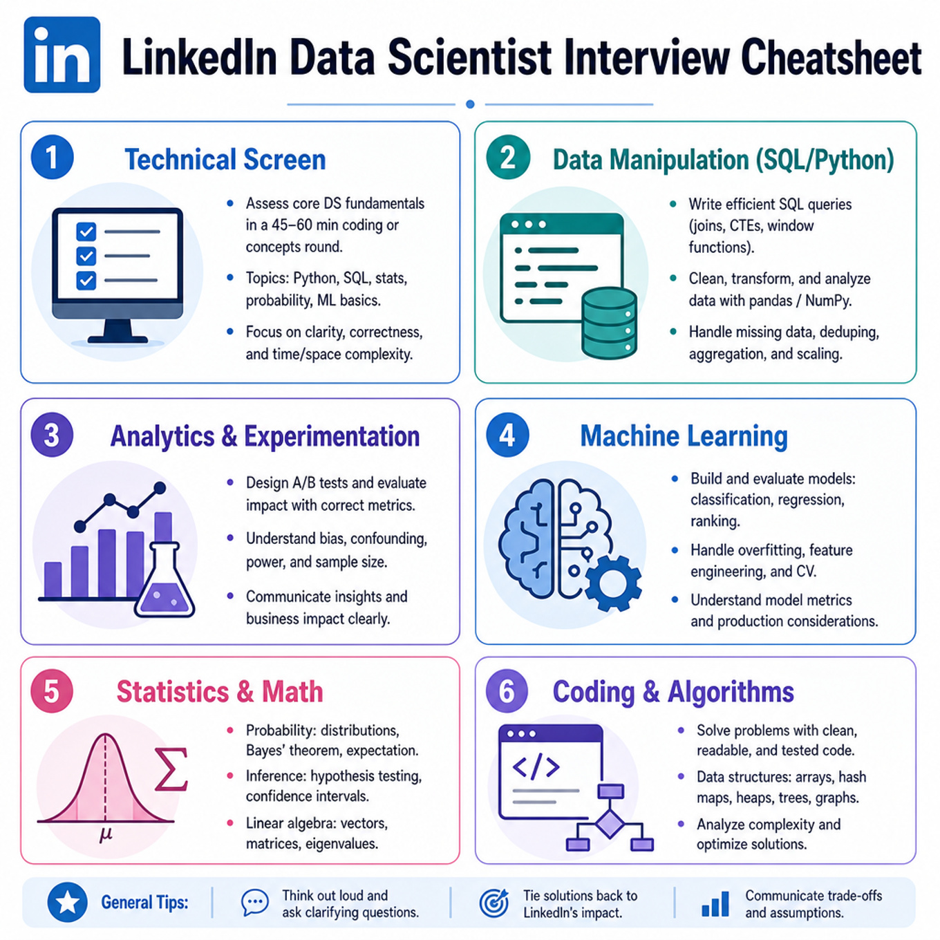
Technical Screen

Data Manipulation (SQL/Python)

What's being tested

These questions test relational data manipulation: joining behavioral logs to entity metadata, filtering by time or action type, deduplicating at the right grain, and aggregating into user-, country-, job-, or continent-level metrics. Interviewers are probing whether you can translate metric definitions into correct SQL or pandas without double-counting or losing edge cases.

Patterns & templates

• Join event logs to dimensions with INNER JOIN or LEFT JOIN; confirm whether missing metadata should drop rows or remain as NULL.

• Deduplicate before aggregating using COUNT(DISTINCT col), drop_duplicates, or a CTE at the metric grain; avoid counting repeated views as unique article types.

• Conditional aggregation with SUM(CASE WHEN action='apply' THEN 1 ELSE 0 END) or COUNT(*) FILTER (WHERE ...) for views, applies, posters, or applicants.

• Window ranking via ROW_NUMBER() OVER (PARTITION BY group_col ORDER BY metric DESC, tie_breaker ASC) for top country, first post, or deterministic tie handling.

• Histogram construction by first computing per-entity values, then grouping those values: user → distinct article types → count of users per diversity bucket.

• Percentage-of-group metrics use metric / SUM(metric) OVER (PARTITION BY group); cast to decimal to avoid integer division in SQL.

• Python equivalent: merge, boolean filters, groupby().agg(), nunique(), rank(method='first'), and value_counts() cover most variants in pandas.

Common pitfalls

Pitfall: Aggregating after a many-to-one or many-to-many join without checking grain can inflate counts, especially for views, applies, or article categories.

Pitfall: Using RANK() when the prompt expects exactly one row per group; prefer ROW_NUMBER() with explicit tie-breakers.

Pitfall: Filtering the wrong table or wrong time column changes the metric definition; clarify whether the date applies to view time, post time, apply time, or metadata creation time.

Practice these

The practice cards below cover the canonical variants — solve all of them and time yourself.

Practice questions

Analytics & Experimentation

• Job Application Funnel Analysis — covered in depth under Onsite below.

• Product Metric Frameworks And Diagnostic Analytics — covered in depth under Onsite below.

• A/B Testing, Power, And Experiment Design — covered in depth under Onsite below.

• Causal Inference, Confounding, And Matching — covered in depth under Onsite below.

Machine Learning

• Recommender Systems, Feed Ranking, And Marketplace Metrics — covered in depth under Onsite below.

• Supervised ML, Imbalance, Overfitting, And Optimization — covered in depth under Onsite below.

Statistics & Math

• Queueing Theory, Probability, And Distributions — covered in depth under Onsite below.

Coding & Algorithms

What's being tested

Interviewers are probing randomized sampling correctness: whether your sample is unbiased, representative, and efficient under constraints like class imbalance, streaming data, or weighted probabilities. For a Data Scientist, the key is connecting algorithmic sampling choices to downstream model bias, metric validity, and generalization.

Patterns & templates

• Reservoir sampling for unknown-length streams — keep k items; replace index randint(0, i) when < k; O(n) time, O(k) space.

• Weighted categorical sampling with prefix sums — build cumulative weights, draw u ~ Uniform(0, total), binary search via bisect; O(log k) per sample.

• Alias method for repeated weighted draws — preprocess probabilities into prob and alias tables; O(k) setup, O(1) sampling; watch normalization errors.

• Stratified sampling for imbalanced labels — sample within each class or segment, then reweight losses/metrics using population prevalence to avoid biased estimates.

• Sample-to-population validation — compare feature distributions using KS tests, standardized mean differences, label prevalence, and segment-level metric drift.

• Model evaluation under imbalance — prefer PR-AUC, recall@k, calibration, cost-weighted loss; accuracy often hides minority-class failure.

• Tree overfitting control — tune max_depth, min_samples_leaf, subsample, colsample_bytree, and validation splits; resampling can amplify leakage.

Common pitfalls

Pitfall: Treating an oversampled training set as if it reflects production prevalence; correct with class weights, prior correction, or population-weighted evaluation.

Pitfall: Implementing weighted sampling with repeated list expansion; it is memory-heavy and fails when weights are large or non-integer.

Pitfall: Forgetting that reservoir sampling replacement probability changes with stream index; every item must end with probability k / n.

Practice these

The practice cards below cover the canonical variants — solve all of them and time yourself.

Practice questions

Onsite

Analytics & Experimentation

What's being tested

Job application funnel analysis tests whether you can turn a high-level metric drop into a disciplined diagnostic plan: define the funnel, localize where the decline occurs, segment intelligently, and separate correlation from likely causation. For LinkedIn, this matters because job applications sit inside a two-sided marketplace: changes that help job seekers may hurt recruiters, and vice versa. Interviewers are probing whether you can reason from metrics like job_views, apply_starts, apply_submits, and qualified_applications to product, ranking, supply, or seasonality explanations without jumping to conclusions. They also want to see whether you can connect descriptive analysis, experiment interpretation, and recommender evaluation into one coherent analytical workflow.

Core knowledge

• Funnel decomposition is the first move: break applications into stages such as job_impressions → job_clicks → apply_starts → apply_submits → recruiter_responses. Track both stage counts and conditional rates, e.g. CTR = job_clicks / job_impressions and submit_rate = apply_submits / apply_starts.

• Metric identity checks prevent vague diagnosis. Total applications can be decomposed as:
  $applications = active\_job\_seekers \times jobs\_seen\_per\_seeker \times view\_rate \times apply\_start\_rate \times submit\_rate$
  A decline can come from demand, supply, ranking, UX friction, or measurement changes.

• Segmentation should be hypothesis-driven, not a fishing expedition. Useful LinkedIn cuts include member_country, device, job_function, seniority, industry, new_vs_returning_job_seekers, job_poster_type, remote_vs_onsite, paid_vs_organic_jobs, and recommended_vs_search traffic.

• Cohort analysis distinguishes a population mix shift from behavioral change. Compare stable cohorts such as members active before the decline, newly active job seekers, or jobs posted in the same week. If only new cohorts degrade, onboarding, acquisition source, or fresh job supply may be implicated.

• Seasonality and calendar effects are major confounders for hiring metrics. Compare year-over-year, same weekday, holiday-adjusted trends, and recruiting cycles. A Monday-to-Friday drop may be normal; a same-day YoY drop in one country or device is more suspicious.

• Causal diagnostics require ruling out concurrent changes. Check launches, ranking changes, notification campaigns, search changes, job posting policy changes, pricing changes, and macro events. The key question is: “What changed at the same time, for the same affected population, and through the same funnel stage?”

• A/B test interpretation should use both primary and guardrail metrics. For a jobs recommender, primary metrics might be apply_submits_per_member or qualified_applications; guardrails include job_hide_rate, short_apply_rate, recruiter_response_rate, and marketplace concentration across employers.

• Statistical significance is not enough. A tiny lift in apply_clicks with a drop in apply_submits may indicate clickbait recommendations. Report effect size, confidence interval, practical impact, and whether the effect persists across key segments.

• Marketplace quality matters more than raw volume. More applications are not automatically better if they are irrelevant. Strong answers consider downstream metrics like qualified_apply_rate, recruiter saves, messages, interviews, or negative feedback from either side.

• Counterfactual thinking separates analysis from reporting. If applications fell after a recommender change, compare exposed versus unexposed users, pre/post trends, and similar unaffected surfaces. Methods may include randomized experiments, difference-in-differences, matched cohorts, or interrupted time-series analysis.

• Instrumentation validation is in-scope from an analytical lens. You should ask whether apply_submit logging changed, whether third-party apply redirects are missing, or whether duplicate applications are counted differently. You are not designing pipelines; you are validating whether the observed metric reflects real user behavior.

• Prioritization of hypotheses should combine impact and plausibility. Start with the largest absolute contributors to the drop, then investigate stage-level changes, affected segments, and known product or market changes. Avoid spending early time on tiny segments with dramatic but low-volume swings.

Worked example

For “Diagnose Job Application Decline: Funnel Analysis and Segmentation”, a strong candidate would first clarify the metric definition: “Are we talking about total submitted applications, unique applicants, applications per active job seeker, or qualified applications?” They would also ask about the time window, comparison baseline, affected geography, and whether the decline is sudden or gradual.

The answer should be organized around four pillars: metric validation, funnel localization, segmentation, and causal hypothesis testing. First, confirm that apply_submit still means the same thing and compare related metrics such as apply_start, external apply redirects, and recruiter-side received applications. Second, decompose the funnel to identify whether the decline starts at job_impressions, job_views, apply_starts, or apply_submits.

Third, segment by traffic source, device, geography, job category, seniority, and member cohort to find whether the problem is broad or concentrated. Fourth, overlay known launches, ranking changes, notification changes, seasonality, and supply-side shifts such as fewer open jobs or more expired postings.

A concrete tradeoff to flag: optimizing for total application volume can degrade marketplace quality if members apply to less relevant jobs. So the investigation should include qualified_application_rate or recruiter engagement, not just raw submits.

A strong close would be: “If I had more time, I’d quantify the contribution of each segment to the total decline, then test the top hypotheses with either experiment readouts or quasi-experimental comparisons against unaffected cohorts.”

A second angle

For “Evaluate 'Job You May Be Interested In' Recommender”, the same funnel logic applies, but the framing shifts from diagnosing a decline to evaluating a ranking system. Instead of starting with “where did the drop happen?”, start with “what user and marketplace outcome should the recommender optimize?” Online metrics might include job_clicks_per_member, apply_starts_per_member, apply_submits_per_member, and qualified_applications, while offline metrics might include precision@k, recall@k, NDCG, or calibration by job category.

The key constraint is that recommender changes often alter both exposure and intent. A model can increase clicks by showing broadly attractive jobs while reducing apply completion if those jobs are poor fits. A strong answer therefore connects recommender quality to downstream funnel health and includes guardrails for employer-side value.

Common pitfalls

Pitfall: Treating total applications as a single metric rather than a decomposable system.

A weak answer says, “Applications dropped, so maybe fewer people are looking for jobs.” A stronger answer decomposes the metric into active seekers, jobs shown, click-through, apply-start rate, and submit rate, then identifies which component explains the decline.

Pitfall: Over-segmenting without a hypothesis.

It is tempting to list every possible dimension: country, device, industry, browser, seniority, acquisition channel, and so on. Interviewers prefer a prioritized segmentation plan: start with dimensions tied to plausible mechanisms and large volume, then drill down only where the contribution to the aggregate decline is material.

Pitfall: Ignoring marketplace quality and downstream outcomes.

For LinkedIn, “more applications” is not always the right answer. If a change increases low-quality applies, recruiters may respond less, jobs may become noisier, and member trust may decline. Include quality metrics such as recruiter response, save rate, interview conversion, or negative feedback.

Connections

Interviewers may pivot from this topic into A/B testing, causal inference, ranking evaluation, or marketplace metrics. Be ready to discuss experiment guardrails, heterogeneous treatment effects, novelty effects, and how to evaluate a recommender when immediate clicks and long-term marketplace quality disagree.

Further reading

• Trustworthy Online Controlled Experiments — Kohavi, Tang, and Xu — practical reference for experiment design, metric selection, guardrails, and interpretation.

• Causal Inference: The Mixtape — Scott Cunningham — accessible treatment of difference-in-differences, event studies, and observational causal reasoning.

• Recommender Systems Handbook — Ricci, Rokach, and Shapira — deeper background on recommender metrics, ranking evaluation, and user-item marketplace tradeoffs.

Practice questions

What's being tested

LinkedIn Data Scientist product cases test whether you can build a metric framework, diagnose metric movement, and design credible analyses without jumping to anecdotes or one-off SQL cuts. The interviewer is probing for structured reasoning: define the product goal, choose primary and guardrail metrics, segment the population, distinguish instrumentation issues from real behavior, and propose experiments or causal analyses. LinkedIn cares because products like the homepage feed, profile, video upload, and B2B offerings are multi-sided systems where short-term engagement, long-term member value, creator incentives, and customer value can diverge. A strong answer shows you can move from “metric went down” to a prioritized diagnostic plan and from “feature looks promising” to an evaluation design that leadership could trust.

Core knowledge

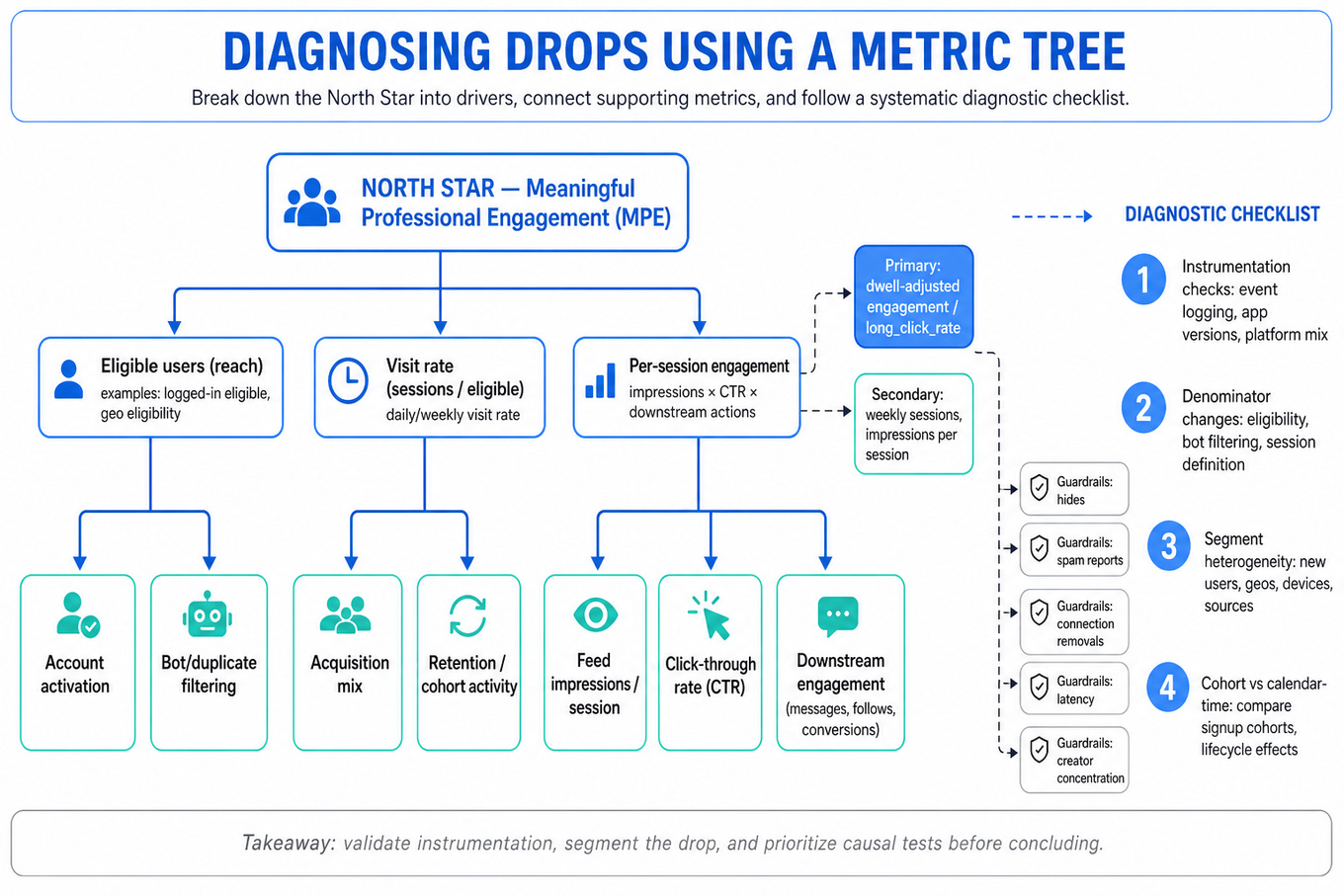
• North Star metrics should reflect durable user or customer value, not just activity. For LinkedIn, examples include meaningful professional engagement, successful job or hiring outcomes, profile completeness that improves match quality, and B2B account adoption. Pair them with input metrics that teams can actually move.

• Metric trees decompose an outcome into drivers. For example, homepage_sessions can be broken into eligible users × visit rate × feed impressions per session × click-through rate × downstream engagement. This helps separate demand changes, ranking quality, UI changes, and content supply effects.

• Primary metrics, secondary metrics, and guardrails serve different purposes. A feed ranking experiment might optimize long_click_rate or dwell-adjusted engagement while guarding against hides, spam reports, connection removals, latency, and creator concentration. Avoid optimizing a single engagement metric that can be gamed by low-quality viral content.

• Diagnostic analytics usually starts with three checks: instrumentation validity, denominator changes, and segment heterogeneity. Before explaining a 10% drop in homepage engagement, verify event logging, app versions, platform mix, bot filtering, logged-in eligibility, and whether the drop is concentrated in new users, geos, devices, or traffic sources.

• Cohort analysis separates lifecycle effects from calendar-time effects. A drop in profile completion may come from more low-intent new signups rather than worse onboarding. Compare signup cohorts by day or week and track completion by age, e.g., day-1, day-7, and day-28 completion rates.

• Funnel metrics should be defined with precise eligibility and time windows. For profile completion: viewed prompt → clicked edit → added field → saved field → reached threshold. Use consistent denominators, such as eligible members exposed to the prompt, not all members, unless the business question is population-level impact.

• Statistical inference depends on the estimand. For “initial video uploads are shorter than later ones,” a paired design compares each creator’s first upload with their own later uploads, reducing between-user variance. A simple estimand is $\Delta = E[length_{later} - length_{first}]$, tested with a paired t-test, Wilcoxon signed-rank test, or regression with creator fixed effects.

• Experiment design requires a clear unit of randomization. For member-facing feed or profile changes, randomize at member level when interference is limited. For B2B products, account-level randomization may be necessary because seats within an account influence each other; otherwise treatment contamination can bias adoption and collaboration metrics.

• Causal diagnosis distinguishes correlation from cause. If homepage engagement dropped after a ranking model launch, compare treated versus unaffected surfaces, pre/post trends, experiment holdouts if available, and segments with different exposure intensity. A difference-in-differences framing is useful when randomized evidence is unavailable:
  $\hat{\tau} = (Y_{treated,post}-Y_{treated,pre})-(Y_{control,post}-Y_{control,pre})$

• Distributional analysis matters for marketplace and enterprise products. In a B2B launch, average seats active per account can hide a few large accounts dominating usage. Inspect account-level adoption, seat-level activation, power-user concentration, retention curves, and percentiles such as p50, p90, and p99.

• Ranking and recommender metrics need both online and offline views. Offline metrics like NDCG, AUC, calibration, and counterfactual replay can catch model regressions, but online metrics measure actual member response. A feed ranking diagnosis should include content inventory, candidate generation coverage, score distribution shifts, and downstream engagement quality.

• Multiple comparisons and peeking can create false discoveries during segmentation. If you inspect 100 segments, some will move by chance. Use pre-specified cuts, false discovery rate control such as Benjamini-Hochberg, or treat exploratory segments as hypotheses requiring validation in a follow-up test.

Worked example

For “Analyze homepage drop and feed ranking,” a strong candidate would first clarify the metric: “Are we seeing a drop in visits, feed impressions, clicks, dwell time, or a composite engagement score, and over what time window versus baseline?” They would also ask whether there were recent launches, logging changes, seasonality events, traffic acquisition shifts, or ranking model changes, while declaring that they will separate data quality from product behavior before diagnosing causality.

The answer should be organized into four pillars: first, validate the metric definition and event logging using raw event counts, platform versions, and comparison to stable metrics such as login_rate; second, decompose the homepage metric tree into user reach, session frequency, feed inventory, impression volume, engagement rate, and downstream quality; third, segment by app platform, geography, new versus existing members, connection graph density, content type, and exposure to the new ranking model; fourth, propose causal tests using experiment logs, launch ramp cohorts, or matched pre/post comparisons.

One tradeoff to flag explicitly is speed versus rigor: in the first few hours, you want high-signal cuts that identify whether the issue is global, platform-specific, or model-exposure-specific; for decision-making, you would prefer randomized holdout or ramp analysis over narrative correlation. A good candidate would avoid saying “the ranking model caused it” just because timing lines up. They would close by saying that if they had more time, they would examine long-term quality metrics such as hides, reports, return visits, and creator-side distribution to ensure any recovery plan does not simply inflate short-term clicks.

A second angle

For “Measure Success of New B2B Product,” the same framework applies, but the unit of analysis changes from individual member sessions to accounts, seats, admins, and buyer value. The metric framework should include acquisition or pilot conversion, account activation, seat adoption, repeated usage, feature depth, retention, and business outcomes such as renewal intent or expansion. Diagnostics must separate account mix from product performance because one large enterprise can dominate aggregate usage. Experimentation is also harder: randomizing individual seats may create spillovers, so account-level tests, phased rollouts, or quasi-experimental comparisons are often more appropriate. The same discipline still holds: define the success metric, decompose it, segment it, validate measurement, and choose the strongest feasible causal design.

Common pitfalls

Pitfall: Treating a metric drop as a single-cause debugging problem.

A tempting answer is “check if the ranking model changed, then roll it back.” That is too narrow for a Data Scientist. A better answer decomposes the metric, validates instrumentation, checks denominator shifts, segments exposure, and then evaluates whether the model change plausibly caused the movement.

Pitfall: Defining metrics that sound good but cannot guide action.

For profile completion, “increase user value” is directionally right but not operational. Stronger metrics include eligible prompt exposure rate, prompt click-through rate, save completion rate, percentage of members reaching all-star or threshold completeness, and downstream outcomes like recruiter profile views or connection acceptance.

Pitfall: Over-indexing on averages.

In B2B and creator/video analyses, averages can be misleading because distributions are skewed. Report medians, percentiles, account-weighted versus seat-weighted views, and cohort-level retention; then explain which weighting matches the decision, such as customer revenue impact versus typical user experience.

Connections

Interviewers may pivot from this topic into A/B testing, causal inference, ranking evaluation, funnel analysis, or statistical hypothesis testing. Be ready to discuss sample size, interference, novelty effects, guardrail metrics, and how you would communicate uncertainty to product and engineering partners.

Further reading

• Trustworthy Online Controlled Experiments, Kohavi, Tang, and Xu — practical reference for experiment design, guardrails, novelty effects, and organizational decision-making.

• Causal Inference: The Mixtape, Scott Cunningham — accessible treatment of difference-in-differences, fixed effects, matching, and causal assumptions.

• Recommender Systems Handbook, Ricci, Rokach, and Shapira — deeper background on recommender evaluation, ranking metrics, and tradeoffs between relevance, diversity, and user value.

Practice questions

What's being tested

LinkedIn is probing whether you can turn a product change into a defensible causal measurement plan, not just compute a p-value after the fact. Strong Data Scientist answers define the estimand, choose primary and guardrail metrics, reason about power, handle segmentation and interference, and explain what to do when results disagree across cohorts. This matters because LinkedIn experiments often affect marketplaces, recommendations, notifications, and social behavior where short-term engagement, long-term member trust, and ecosystem health can move in different directions. Interviewers are looking for statistical rigor plus product judgment: can you design an experiment that answers the business question without overclaiming?

Core knowledge

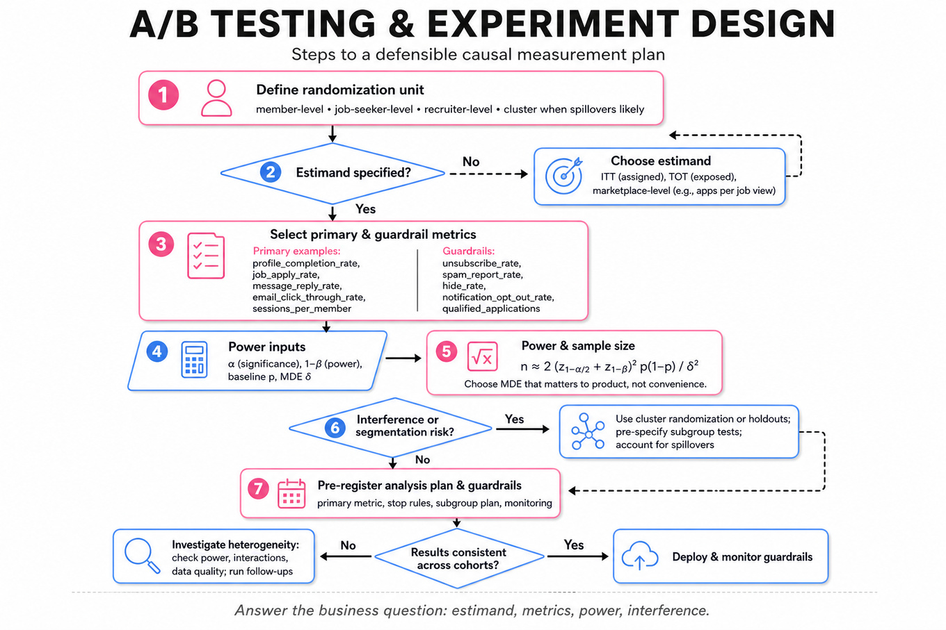
• A/B testing estimates a causal effect by randomizing units into treatment and control. Define the unit first: member-level randomization for profile nudges, job-seeker-level randomization for job recommendations, recruiter-level randomization for hiring tools, or cluster randomization when network spillovers are likely.

• Estimand clarity prevents ambiguous conclusions. State whether you want the intent-to-treat effect on all assigned users, the treatment-on-treated effect among exposed users, or a marketplace-level effect such as applications per job view. For most product experiments, ITT = E[Y | assigned treatment] - E[Y | assigned control] is the safest default.

• Primary metrics should map directly to the product objective and be chosen before launch. Examples: profile_completion_rate, job_apply_rate, message_reply_rate, email_click_through_rate, or sessions_per_member. Pair them with guardrail metrics like unsubscribe_rate, spam_report_rate, hide_rate, notification_opt_out_rate, or downstream quality such as qualified_applications.

• Power analysis links detectable effect, sample size, variance, and significance. For a two-sample test on proportions with equal allocation, a useful approximation is:
  $n \approx \frac{2(z_{1-\alpha/2} + z_{1-\beta})^2 p(1-p)}{\delta^2}$
  where $p$ is baseline rate, $\delta$ is the minimum detectable effect, $\alpha$ is false positive rate, and $1-\beta$ is power.

• Minimum detectable effect should be product-relevant, not just statistically convenient. If profile_completion_rate is 40%, a 0.05 percentage-point lift may be detectable at LinkedIn scale but operationally meaningless; a 1–2 percentage-point lift may justify launch depending on downstream value.

• Variance reduction improves sensitivity without increasing traffic. CUPED uses a pre-experiment covariate $X$ to adjust outcome $Y$:
  $Y' = Y - \theta(X - \bar{X}), \quad \theta = \frac{\operatorname{Cov}(Y, X)}{\operatorname{Var}(X)}$
  This is useful for stable member behaviors like historical engagement, prior apply rate, or previous message response rate.

• Sequential testing is risky if you repeatedly peek and stop when p-value < 0.05. Use pre-planned methods such as alpha spending, group sequential tests, or always-valid confidence intervals. Otherwise, “checking every day” inflates false positives and produces fragile launch decisions.

• Multiple testing matters when examining many segments, metrics, or variants. If you test by city, industry, seniority, and device, some significant results will occur by chance. Use Bonferroni correction, Benjamini-Hochberg false discovery rate, or declare subgroup analyses exploratory unless pre-registered.

• Heterogeneous treatment effects are common on LinkedIn. A job recommendation update may help active job seekers but hurt passive candidates; an online indicator may increase replies for close connections but feel invasive for weak ties. Report both aggregate effect and key pre-specified segment effects with confidence intervals.

• Simpson’s paradox appears when aggregate and segment-level results conflict due to composition differences. If treatment has more high-activity members or more large cities, aggregate metrics can reverse. Diagnose by checking randomization balance, stratifying by baseline covariates, and estimating weighted or regression-adjusted effects.

• Interference and network effects violate standard A/B assumptions. Messaging, feed ranking, and job marketplaces can have spillovers: one member’s treatment changes another member’s experience. Consider cluster randomization, geo-level tests, switchback designs, or marketplace-side guardrails when interactions are material.

• Experiment validity checks come before interpreting impact. Verify sample ratio mismatch, exposure logging consistency, pre-treatment covariate balance, missing outcome rates, and novelty effects. A statistically significant lift is not credible if assignment proportions are off or exposure only happened for a biased subset.

Worked example

For Design Experiments for Email Campaign & Messaging Update, a strong candidate starts by clarifying whether the email campaign and messaging update are independent product surfaces or could interact through member attention. In the first 30 seconds, they would ask: “What is the primary business goal: more conversations, more replies, more sessions, or downstream job outcomes? Are we optimizing member engagement, recruiter success, or both? Can the same member receive both treatments?” Then they would propose a factorial design if both changes can run simultaneously: control, email only, messaging only, and email plus messaging.

The answer skeleton should have four pillars: metric definition, randomization and exposure, power and duration, and interpretation. For metrics, they might choose message_reply_rate or qualified_conversation_starts as primary, with guardrails like unsubscribe_rate, spam_report_rate, and notification_disable_rate. For design, they would randomize at member level if spillovers are limited, but consider cluster or sender-level randomization if messaging behavior creates peer effects. For power, they would estimate baseline conversion, minimum detectable effect, expected eligible traffic, and whether interaction effects require a larger sample than main effects.

A specific tradeoff to flag: a factorial design is efficient for detecting main effects, but detecting the email-by-messaging interaction may require substantially more sample, so the team should decide whether interaction is a must-have decision criterion. They should also mention sequential monitoring: daily dashboards are fine for data quality and guardrails, but launch decisions should follow a pre-specified stopping rule. A strong close would be: “If I had more time, I’d add heterogeneity analysis by member activity, connection strength, and prior email engagement, but I’d label those as exploratory unless we powered them in advance.”

A second angle

For Resolve Conflicting A/B Test Results in Cities, the same principles apply, but the center of gravity shifts from initial design to causal diagnosis. The candidate should not simply average city-level lifts or pick the largest city result; they should ask whether the estimand is the national member-level effect, the average city effect, or the effect for a launch market. Conflicts across cities may reflect heterogeneous treatment effects, seasonality, sample imbalance, different baseline usage, or marketplace density. A strong answer would compare stratified estimates, check covariate balance within cities, compute a pooled regression with city fixed effects, and explain whether the decision should be global launch, targeted launch, or follow-up experiment. The key difference is that segmentation is no longer just a readout; it directly affects the causal interpretation and product rollout decision.

Common pitfalls

Pitfall: Treating statistical significance as the launch criterion.

A tempting answer is: “If p < 0.05, ship; otherwise don’t.” That misses effect size, metric hierarchy, guardrails, power, and business value. A better answer says launch requires a practically meaningful lift on the primary metric, no unacceptable harm to guardrails, and credible experimental validity.

Pitfall: Ignoring the randomization unit.

Many candidates say “randomly split users 50/50” without considering spillovers. For recommendations, messaging, and online indicators, one treated member can affect another member’s outcomes. Interviewers expect you to call out interference risk and propose member-level, sender-level, cluster-level, or marketplace-level randomization depending on the product surface.

Pitfall: Over-indexing on formulas without product framing.

Power equations are useful, but a Data Scientist must also justify the baseline, MDE, eligible population, ramp plan, and decision rule. Saying “we need larger sample size for smaller effects” is not enough; stronger answers quantify the tradeoff and connect it to DAU, conversion rate, experiment duration, and launch cost.

Connections

Interviewers may pivot from this topic into causal inference, especially matching, difference-in-differences, or instrumental variables when randomization is unavailable. They may also move into metric design, recommender evaluation, marketplace health, or diagnosing experiment anomalies such as sample ratio mismatch and segment-level reversals.

Further reading

• Trustworthy Online Controlled Experiments by Kohavi, Tang, and Xu — Practical reference for experiment design, pitfalls, metrics, and interpretation at internet scale.

• Controlled experiments on the web: survey and practical guide by Kohavi, Henne, and Sommerfield — Classic paper on online experimentation failure modes, power, and organizational practices.

• Experimentation Works by Stefan Thomke — Useful for understanding how rigorous experimentation connects to product decision-making and organizational learning.

Practice questions

What's being tested

Interviewers are probing whether you can separate causal impact from correlation when product behavior changes outside a clean randomized experiment. For a LinkedIn Data Scientist, this matters because product decisions often depend on metrics like job_applications, apply_start_rate, notification_ctr, profile_views, or sessions_per_member, where user mix, market conditions, ranking changes, and seasonality can all confound the observed trend. You are expected to reason through confounding, selection bias, heterogeneous treatment effects, and Simpson’s paradox, then propose an analysis that estimates the right causal quantity. Strong answers define the estimand, diagnose bias, segment intelligently, and communicate uncertainty rather than overclaiming.

Core knowledge

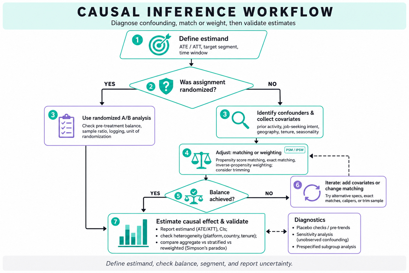
• Causal inference starts with an estimand: what effect are we trying to estimate, for whom, over what time window? Common estimands include ATE $E[Y(1)-Y(0)]$, ATT $E[Y(1)-Y(0)\mid T=1]$, and segment-specific effects such as impact on new job seekers in US metro areas.

• Confounding occurs when a variable affects both treatment assignment and outcome. If active job seekers are more likely to receive an email and also more likely to apply, raw email recipients versus non-recipients will overstate impact unless you adjust for prior activity, job-seeking intent, geography, seniority, and seasonality.

• Randomized A/B tests solve confounding in expectation because treatment assignment is independent of potential outcomes: $T \perp (Y(0),Y(1))$. Still, you must check sample ratio mismatch, pre-treatment balance, logging gaps, interference between users, novelty effects, and whether the randomization unit matches the metric unit.

• Simpson’s paradox happens when aggregate results reverse after conditioning on a key variable. For example, a redesign may look negative overall but positive in every city if traffic shifted toward cities with lower baseline application rates. Always compare aggregate, stratified, and reweighted estimates.

• Heterogeneous treatment effects are expected in marketplace products. A job-application redesign may help mobile users but hurt desktop users, or help entry-level seekers but hurt senior roles. Pre-specify critical cuts like country, platform, member tenure, job-seeker intent, and recruiter/job supply density to avoid cherry-picking.

• Propensity score matching estimates $e(X)=P(T=1\mid X)$ using pre-treatment covariates, often via logistic regression, XGBoost, or generalized boosted models. Match treated and control users with similar $e(X)$, then estimate outcomes within the matched sample. The key assumption is conditional ignorability: $(Y(0),Y(1)) \perp T \mid X$.

• Common support is mandatory for matching. If redesigned users have propensity scores near 0.95 and control users are mostly near 0.10, no statistical method can reliably infer counterfactuals for the treated group. Trim non-overlap regions and report that the estimate applies only to the matched population.

• Covariate balance matters more than propensity model accuracy. After matching or weighting, compare standardized mean differences:
  $\text{SMD}=\frac{\bar X_T-\bar X_C}{s_{\text{pooled}}}$
  A common target is absolute SMD < 0.1 for major covariates such as prior applications, sessions, platform, geography, and member age.

• Inverse probability weighting uses weights $w_i=T_i/e(X_i)+(1-T_i)/(1-e(X_i))$ to create a pseudo-population balanced on covariates. It can use more data than matching but becomes unstable when propensity scores are near 0 or 1, so stabilized weights and trimming are often needed.

• Difference-in-differences compares pre/post changes between treated and control groups:
  $\hat\delta=(\bar Y_{T,post}-\bar Y_{T,pre})-(\bar Y_{C,post}-\bar Y_{C,pre})$
  It relies on parallel trends, which you should probe with pre-period trend plots, placebo tests, and event-study coefficients.

• Event studies estimate dynamic effects around launch time and help distinguish immediate product impact from pre-existing drift. A typical model includes user or segment fixed effects, date fixed effects, and treatment-relative-time indicators; significant pre-period coefficients are evidence against a causal interpretation.

• Metric decomposition is essential for diagnosing declines. For job_applications, break the funnel into job_impressions, job_clicks, apply_starts, apply_submits, and completion rate. Then segment by traffic source, country, platform, job category, member intent, and supply-side changes before attributing the drop to a product change.

Worked example

For Estimate Redesign Impact Using Propensity Score Matching, a strong first 30 seconds would clarify whether the redesign was rolled out non-randomly, what the treatment unit is, what outcome window defines impact, and whether the target estimand is ATE or ATT. I would say: “If users self-selected or were selected by market/platform, the raw difference in application rate is biased; I’ll estimate the effect on treated users if comparable untreated users exist.” The answer skeleton would have four pillars: define outcome and pre-treatment covariates, estimate propensity scores using only variables observed before exposure, assess common support and balance, then estimate the treatment effect with uncertainty.

I would include covariates like prior job_applications, sessions_per_week, platform, country, industry, seniority, job-seeker intent signals, acquisition channel, and calendar week. After matching, I would report balance using standardized mean differences rather than saying the model has high AUC because prediction quality is not the causal objective. A specific tradeoff is nearest-neighbor matching versus weighting: matching is easier to explain and inspect, but weighting preserves more observations and may have lower variance if weights are stable. I would explicitly flag that unobserved confounders, such as a member’s offline urgency to change jobs, can still bias the estimate. I’d close with: “If I had more time, I’d run sensitivity checks, compare to difference-in-differences or an event study, and recommend a randomized holdout for future redesign launches.”

A second angle

For Resolve Conflicting A/B Test Results in Cities, the same causal idea appears inside an experiment rather than an observational rollout. The trap is to average all cities and declare a single winner without noticing that treatment exposure, baseline application rates, or user mix differ sharply by city. Because randomization protects the overall estimate but not necessarily every underpowered segment, I would first define whether the decision is global impact, city-level impact, or impact on a weighted business population. Then I would inspect stratified effects, confidence intervals, traffic allocation, and whether the aggregate result is being driven by composition shifts. If city is a pre-treatment moderator, I might report both the overall ATE and a city-reweighted estimate aligned to the launch population.

Common pitfalls

Pitfall: Treating adjustment as a magic fix.

A tempting answer is “control for all variables in a regression” or “use propensity score matching” without naming assumptions. Better answers state which variables are pre-treatment confounders, exclude post-treatment mediators, check balance/common support, and acknowledge that unobserved confounding remains possible.

Pitfall: Over-segmenting until the story looks clean.

When faced with Simpson’s paradox or city-level conflicts, candidates often slice by dozens of dimensions and pick the most intuitive pattern. A stronger approach distinguishes pre-specified diagnostic segments from exploratory cuts, uses confidence intervals or multiple-testing caution, and connects segments back to a causal graph or product mechanism.

Pitfall: Communicating only the statistical method, not the decision.

A DS answer should not end at “the ATT is 1.8%.” Explain whether that translates into more job_applications, whether it affects guardrails like unsubscribe_rate or session_depth, which population the estimate covers, and whether the evidence is strong enough to launch, pause, or run a cleaner experiment.

Connections

Interviewers may pivot from here into A/B testing design, metric decomposition, regression adjustment, instrumental variables, synthetic controls, or marketplace interference. For LinkedIn-style products, also expect connections to ranking evaluation, notification experiments, job-seeker funnel metrics, and cohort-based trend diagnosis.

Further reading

• Rosenbaum and Rubin, “The Central Role of the Propensity Score in Observational Studies for Causal Effects” — the foundational paper behind propensity score matching and balance diagnostics.

• Scott Cunningham, Causal Inference: The Mixtape — practical coverage of matching, difference-in-differences, event studies, and causal assumptions.

• Kohavi, Tang, and Xu, Trustworthy Online Controlled Experiments — strong reference for experimentation pitfalls, heterogeneity, and trustworthy metric interpretation.

Practice questions

Machine Learning

What's being tested

LinkedIn is probing whether a Data Scientist can reason about recommendation quality, feed ranking, and marketplace outcomes beyond “optimize clicks.” Strong answers connect user behavior, model labels, online experiments, offline evaluation, and long-term ecosystem health. The interviewer is looking for judgment: which metrics matter, how to diagnose metric movement, how to separate ranking effects from instrumentation or traffic-mix effects, and how to evaluate tradeoffs across members, creators, recruiters, and job seekers. For LinkedIn specifically, recommendations shape core surfaces like the homepage feed, jobs, notifications, and creator distribution, so small ranking changes can affect engagement, trust, retention, and marketplace liquidity.

Core knowledge

• Multi-stage recommender systems usually separate candidate generation, ranking, and re-ranking. A DS should know the metric purpose of each stage: candidate generation targets recall, ranking targets relevance or utility, and re-ranking enforces diversity, freshness, policy constraints, or marketplace balance.

• Label choice is the first major modeling decision. Optimizing CTR favors curiosity and clickbait; optimizing dwell_time may favor passive consumption; optimizing apply_rate, connection_accept_rate, or long_click_rate better captures downstream value. A common utility formulation is:
  $\text{score}(u, i) = P(\text{action} \mid u,i) \times \text{value(action)} - \text{cost}(u,i)$

• Offline metrics should match the stage being evaluated. Use Recall@K or HitRate@K for retrieval, NDCG@K or MAP@K for ranked relevance, and calibration metrics such as Brier score or reliability curves when predicted probabilities are used directly in ranking or bidding-like tradeoffs.

• Online metrics need a hierarchy: a primary success metric, guardrails, and diagnostics. For feed, primary metrics might include sessions_per_member, feed_engaged_sessions, or quality_weighted_actions; guardrails include hide_rate, unfollow_rate, report_rate, negative_feedback_rate, creator distribution, and member retention.

• Marketplace recommenders require two-sided metrics. For Jobs You May Be Interested In, candidate-side metrics include job_click_rate, save_rate, apply_start_rate, apply_completion_rate, and job-seeker retention. Employer-side metrics include qualified applicants per job, recruiter response rate, fill probability, and applicant quality.

• Experiment design must account for interference. Feed and creator recommendations can violate the stable unit treatment value assumption because changing exposure for one member changes impressions available to others. For heavy supply-side interactions, consider creator-level, job-level, geo-level, or cluster-randomized designs, or interpret member-level A/B tests as partial-equilibrium effects.

• Causal diagnosis starts by decomposing a metric. If homepage_sessions drops, break it into eligible users, visits, feed loads per visit, items shown per load, impressions, actions per impression, and downstream retention. A useful decomposition is:
  $\text{actions} = \text{users} \times \text{sessions/user} \times \text{impressions/session} \times \text{actions/impression}$

• Segmentation is not optional in ranking problems. Always inspect new versus tenured members, job seekers versus non-job seekers, creators versus consumers, mobile versus desktop, geography, language, network size, and cold-start users. Aggregate gains can hide harm to sparse-history members or niche content producers.

• Cold start changes both modeling and evaluation. For new users, rely more on declared profile fields, onboarding intents, location, industry, skills, and popularity priors. For new items, evaluate exposure fairness and early engagement separately, because historical engagement labels are missing or biased by prior ranking.

• Position bias contaminates naive relevance labels. Items ranked high receive more clicks regardless of quality. A DS should mention randomized exploration buckets, inverse propensity scoring, or interleaving when estimating unbiased relevance:
  $\hat{R}_{IPS} = \frac{1}{n}\sum_i \frac{\mathbb{1}(\text{clicked}_i) \cdot y_i}{p_i}$
  where $p_i$ is the probability the item was shown in that position.

• Short-term and long-term metrics can conflict. A model increasing CTR may reduce trust through low-quality viral posts, stale content, or irrelevant job recommendations. LinkedIn-style surfaces often need composite objectives that include satisfaction surveys, negative feedback, diversity, creator health, and repeat usage after 7 or 28 days.

• Model evaluation is not the same as product evaluation. A larger AUC or NDCG@10 does not guarantee better business outcomes if labels are misaligned, exploration changes exposure, or the new ranker shifts traffic toward low-value actions. A strong DS ties offline lifts to expected online movement, then validates with controlled experiments.

Worked example

For “Evaluate 'Job You May Be Interested In' Recommender”, a strong candidate would first clarify the recommendation surface: email, homepage module, job tab, or notification, because user intent and acceptable frequency differ. They would ask what the current goal is: more applications, more qualified applications, better job-seeker retention, or employer success. Then they would frame the answer around four pillars: offline relevance evaluation, online A/B testing, marketplace guardrails, and diagnostic segmentation.

The offline section would include Recall@K, NDCG@K, and calibration for predicted apply probability, but would explicitly warn that historical applications are biased by previous exposure. The online experiment would define a primary metric such as qualified apply_completion_rate per eligible member, with guardrails like notification opt-outs, irrelevant-job feedback, employer response rate, and application quality. A key tradeoff to flag is volume versus quality: a ranker can increase applications by showing easy-apply jobs more often while lowering recruiter satisfaction or job-seeker trust. The candidate should also segment by active job seekers, passive candidates, geography, seniority, industry, and cold-start members, because relevance signals vary heavily across those cohorts. They could close by saying: “If I had more time, I would add long-term outcomes like interview starts, hires, 28-day job-seeker retention, and employer repeat posting, because immediate apply clicks are only a proxy.”

A second angle

For “Analyze homepage drop and feed ranking”, the same recommender-system thinking applies, but the framing is diagnostic rather than evaluative. Instead of designing success metrics for a planned experiment, the candidate needs to isolate whether the drop came from traffic mix, logging, eligibility, ranking quality, content supply, or user behavior after exposure. A strong answer decomposes homepage_engagement into users, sessions, feed loads, impressions, ranking positions, action rates, and negative feedback. The ranking angle appears when checking whether specific content types, creators, or member cohorts lost distribution after a model or policy change. The best candidates also separate “true product decline” from measurement artifacts by validating metric consistency across independent signals, without drifting into pipeline implementation details.

Common pitfalls

Pitfall: Optimizing only CTR and calling it recommendation quality.

Clicks are easy to measure but often reward sensational, stale, or low-value content. A better answer distinguishes immediate engagement from long-term member value using dwell_time, meaningful interactions, hides, reports, survey satisfaction, return rate, and marketplace outcomes.

Pitfall: Giving an ML architecture answer when the interviewer asked for DS evaluation.

For a Data Scientist, the core is not how to serve embeddings or tune retrieval latency. Stay focused on label definition, offline-to-online metric alignment, experiment design, causal interpretation, cohort cuts, and whether the recommender improves the LinkedIn ecosystem.

Pitfall: Treating aggregate experiment lift as sufficient.

A feed or jobs recommender can show a positive average treatment effect while harming new members, small creators, niche job categories, or employers receiving lower-quality applicants. Strong candidates proactively discuss heterogeneity, guardrails, multiple testing discipline, and whether the launch decision changes by segment.

Connections

Interviewers may pivot from here into A/B testing, causal inference, metric design, ranking evaluation, or marketplace analytics. Be ready to discuss interference, novelty effects, counterfactual evaluation, power analysis, and how to choose between competing north-star and guardrail metrics.

Further reading

• Recommender Systems Handbook, Ricci, Rokach, and Shapira — comprehensive reference for retrieval, ranking, evaluation, and recommender tradeoffs.

• Deep Neural Networks for YouTube Recommendations, Covington et al. — classic multi-stage recommendation architecture with practical label and ranking considerations.

• Unbiased Offline Evaluation of Contextual-bandit-based News Article Recommendation Algorithms, Li et al. — foundational paper for counterfactual evaluation and propensity-based reasoning in recommendation systems.

Practice questions

What's being tested

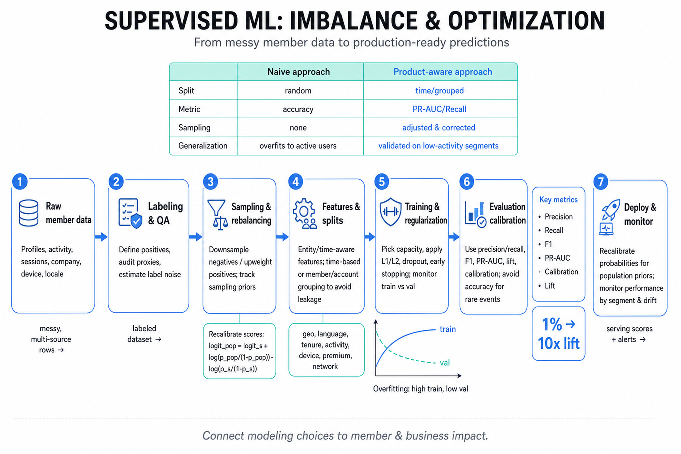
Interviewers are probing whether you can build and evaluate supervised learning models when the data is messy, skewed, and product-relevant rather than textbook-clean. For LinkedIn Data Scientists, this matters because many valuable prediction tasks are rare-event problems: identifying sales professionals, predicting product adoption, detecting low-frequency bad experiences, or ranking member-job interactions. You’re expected to reason about class imbalance, sampling bias, overfitting, regularization, and evaluation metrics in a way that connects model behavior to business and member impact. Strong answers show you can move between statistical fundamentals, practical modeling choices, and decision-quality evaluation.

Core knowledge

• Class imbalance means the target classes have very unequal prevalence, such as 1% positives and 99% negatives. Accuracy becomes misleading: a classifier that predicts all negatives gets 99% accuracy but has zero recall for the minority class. Use precision, recall, F1, PR-AUC, lift, and calibration-aware metrics instead.

• Sampling strategy changes both training dynamics and probability interpretation. Downsampling negatives can make training faster and improve signal visibility, but predicted probabilities need correction if the sample class prior differs from production. If $p_s(y=1)$ is the sampled prior and $p(y=1)$ is the population prior, recalibrate before using scores as probabilities.

• Representative sampling is not just random rows. For LinkedIn-style member data, check representativeness across geography, language, tenure, industry, activity level, device, premium status, and network size. A model trained on highly active members may generalize poorly to casual members, even if aggregate class balance looks fine.

• Train/validation/test splitting must match the deployment question. Use time-based splits when predicting future behavior from past signals, because random splits can leak future engagement patterns. Use member-level or account-level grouping when multiple rows per entity exist; otherwise, the model may memorize user-specific patterns.

• Label quality often dominates algorithm choice. For “Identify Sales Professionals,” self-reported titles, profile text, recruiter tags, company pages, and behavioral signals can all be noisy proxies. Define positives and negatives carefully, audit ambiguous labels, and consider a “silver label” approach with manual validation for a high-confidence evaluation set.

• Logistic regression estimates $P(y=1\mid x)=\sigma(w^\top x+b)=\frac{1}{1+e^{-(w^\top x+b)}}.$ It is equivalent to a one-layer neural network with a sigmoid output trained using binary cross-entropy: $-\left[y\log(\hat p)+(1-y)\log(1-\hat p)\right].$ It is interpretable, strong for sparse features, and a good baseline.

• Tree-based models such as RandomForest, XGBoost, and LightGBM handle nonlinearities and feature interactions well, but can overfit if depth, leaves, or boosting rounds are too large. Control complexity using max_depth, min_child_weight, min_samples_leaf, subsample, colsample_bytree, learning rate, and early stopping.

• Overfitting shows up when validation performance degrades while training performance keeps improving. In imbalanced settings, it can be hidden if you only monitor accuracy or ROC-AUC. Compare train versus validation PR-AUC, precision at fixed recall, recall at fixed precision, and calibration curves by segment.

• Regularization trades variance for bias. L2 regularization adds $\lambda\lVert w\rVert_2^2$ and shrinks coefficients smoothly; L1 regularization adds $\lambda\lVert w\rVert_1$ and can drive coefficients to zero, acting as feature selection. L1 may be useful for high-dimensional sparse text or profile features, but it can arbitrarily select one of many correlated features.

• Optimization matters for explaining model training, not just implementation. Gradient descent updates parameters by moving opposite the loss gradient: $w_{t+1}=w_t-\eta\nabla L(w_t)$. Adam adapts learning rates using first and second moment estimates of gradients, often converging faster than vanilla SGD, though learning rate and regularization still need validation.

• Threshold selection should be tied to product cost. If false positives annoy members or sales teams, optimize precision at an acceptable recall. If missing true positives is costly, optimize recall subject to precision. Ranking use cases may care more about precision@k, recall@k, lift over random, or incremental business value than a global classification threshold.

• Calibration is essential when scores drive decisions like opportunity sizing or resource allocation. A model can rank well but produce poorly calibrated probabilities. Use reliability plots, Brier score, Platt scaling, isotonic regression, or segment-level calibration checks before interpreting “20% probability of adoption” literally.

Worked example

For Train with imbalanced sampled data, a strong candidate would first clarify the prediction target, positive-class prevalence in the population, how the sample was drawn, and whether the output is used for ranking, classification, or calibrated probability estimation. In the first 30 seconds, you might say: “I’d separate three concerns: whether the training sample is representative, how imbalance affects learning, and which metric matches the product decision.” The answer skeleton should have four pillars: audit sample-to-population differences, choose an imbalance strategy, train with overfitting controls, and evaluate on an untouched population-like test set.

For sampling, you would compare distributions of key covariates between sampled and population data, such as member activity, region, seniority, industry, and historical engagement. For imbalance, you could discuss class weights, downsampling, upsampling, or algorithms that support weighted loss, while noting that resampling affects probability calibration. For overfitting, you would propose time-based validation, cross-validation where appropriate, early stopping for boosted trees, limiting tree depth, and monitoring train-validation gaps on PR-AUC or precision at target recall. A specific tradeoff to flag: downsampling negatives improves speed and minority signal, but may discard useful variation among negatives and requires prior correction if probabilities are used. You could close with: “If I had more time, I’d run segment-level error analysis and calibration checks, because overall PR-AUC can hide failure on smaller but important member cohorts.”

A second angle

For Explain Logistic Regression, Backprop, and Adam, the same ideas appear through the lens of model fundamentals rather than sampling design. Logistic regression is a supervised binary classifier trained by minimizing binary cross-entropy, and class imbalance can be handled by weighting the positive class more heavily in the loss. Backpropagation is simply the chain rule used to compute gradients of that loss with respect to model parameters; in logistic regression, the gradient has a simple form, but the same principle extends to deeper networks. Adam changes the optimization path by adapting step sizes per parameter, but it does not solve bad labels, leakage, poor metrics, or sampling bias. The best answer connects the math to practice: explain the formula, then say how you would validate convergence, regularization, threshold choice, and calibration.

Common pitfalls

Pitfall: Optimizing accuracy on an imbalanced dataset.

This is the classic analytical mistake. If positives are rare, a high-accuracy model can be useless for the actual product decision. A better answer names the operating point: for example, “I’d optimize precision at 80% recall” or “I’d compare models using PR-AUC and lift in the top decile.”

Pitfall: Saying “just oversample the minority class” without discussing bias or calibration.

Oversampling can help the learner see enough positive examples, but it does not create new information unless paired with careful validation. If the sampled class prior differs from the production prior, raw model probabilities are not directly interpretable. Strong candidates explicitly distinguish ranking quality from probability calibration.

Pitfall: Giving a model-shopping answer instead of a diagnostic answer.

Jumping straight to XGBoost or a neural network can sound shallow if you ignore labels, leakage, sample representativeness, and evaluation design. Interviewers usually reward a structured debugging mindset: define the target, inspect the data-generating process, choose metrics, establish a simple baseline, then justify more complex models only if they improve validated decision quality.

Connections

Interviewers can pivot from here into experiment design, especially how you would validate that a model-driven product change improves member outcomes through an A/B test. They may also move into ranking evaluation, causal inference, feature leakage, calibration, or cohort-level error analysis, all of which are natural extensions for a Data Scientist working on LinkedIn products.

Further reading

• The Elements of Statistical Learning — Deep reference for supervised learning, regularization, trees, boosting, and model assessment.

• Imbalanced Learning: Foundations, Algorithms, and Applications — Focused treatment of imbalanced classification, sampling, cost-sensitive learning, and evaluation.

• Deep Learning, Chapter 8: Optimization for Training Deep Models — Clear explanation of gradient-based optimization, momentum, adaptive methods, and practical training issues.

Practice questions

Statistics & Math

What's being tested

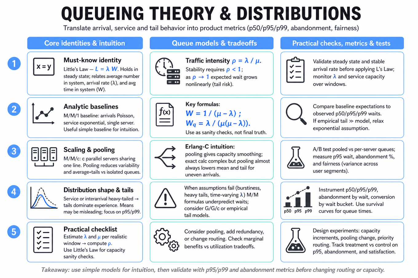
Interviewers are probing whether you can translate messy product or operational behavior into stochastic models, reason about waiting time, arrival rates, service rates, and distribution shape, then connect the math back to user-facing metrics. For a LinkedIn Data Scientist, this matters in contexts like member support routing, recruiter response delays, notification delivery timing, feed/ranking latency as experienced by users, or marketplace matching where queues and heavy-tailed behavior affect fairness and satisfaction. The interviewer is not looking for infrastructure design; they want to see whether you can choose reasonable assumptions, derive or approximate expectations, identify when assumptions fail, and propose empirical validation using metrics like p50, p95, p99, conversion, abandonment, or satisfaction scores. Strong answers combine formulas with interpretation: what does a lower mean wait imply, when does the tail dominate, and how would you test whether a queueing change improved the member experience?

Core knowledge

• Little’s Law is the must-recall queueing identity: $L = \lambda W$ where $L$ is average number in system, $\lambda$ is average arrival rate, and $W$ is average time in system. It is broadly applicable under steady state, regardless of arrival or service-time distribution, as long as the system is stable.

• Traffic intensity or utilization is usually $\rho = \lambda / \mu$ for a single-server queue with arrival rate $\lambda$ and service rate $\mu$. Stability requires $\rho < 1$; as $\rho \to 1$, expected wait grows nonlinearly, so “only 90% utilized” can still mean painful tail waits.

• In an M/M/1 queue, arrivals are Poisson, service times are exponential, and there is one server. Key formulas include $W = 1/(\mu-\lambda)$ for time in system and $W_q = \lambda/(\mu(\mu-\lambda))$ for time waiting before service. These are useful baselines, not universal truths.

• In an M/M/c queue, there are $c$ parallel servers sharing one line. Exact Erlang-C calculations can be complex, but the practical intuition is clear: pooling capacity reduces variability and usually lowers average and tail wait compared with separate isolated queues, especially when arrivals are uneven.

• Single queue versus multiple queues is a fairness and variance tradeoff. A single pooled queue generally minimizes expected wait and reduces “wrong line” risk; multiple queues may improve specialization, perceived autonomy, or routing quality if different servers have different skill or service-time distributions.

• Service-time variability matters as much as mean service time. With a G/G/1 queue, Kingman’s approximation says $W_q \approx \frac{\rho}{1-\rho} \cdot \frac{c_a^2+c_s^2}{2} \cdot E[S]$ where $c_a^2$ and $c_s^2$ are squared coefficients of variation for arrivals and service. High variability inflates waits.

• Poisson processes model independent random arrivals with rate $\lambda$, where counts follow $N(t)\sim \text{Poisson}(\lambda t)$ and interarrival times follow $\text{Exponential}(\lambda)$. They are a starting point for arrivals, but real product traffic often has time-of-day seasonality, bursts, and correlated behavior.

• Exponential distributions are memoryless: $P(X>s+t\mid X>s)=P(X>t)$. This property makes Markov-chain derivations tractable, but it is often unrealistic for human task times, which may be lognormal, gamma, Weibull, or heavy-tailed depending on the workflow.

• Waiting for patterns in Bernoulli trials is commonly solved with recurrence equations or a small Markov chain. For example, the expected number of fair coin flips until two consecutive heads is $6$, not $4$, because partial progress can be lost after a tail.

• Mean, median, and mode separate sharply under skewed distributions. For right-skewed data such as response times, income, follower counts, or session lengths, typically mean $>$ median $>$ mode. Reporting only the mean can hide the experience of most users or obscure tail-risk segments.

• Heavy-tailed and power-law distributions appear in network degree, creator impressions, job applications per posting, and engagement counts. A small number of members or entities can dominate totals, so robust summaries like median, trimmed mean, quantiles, log-scale plots, and segment-level metrics are often more informative.

• L1 versus L2 estimators connect distributional assumptions to modeling choices. Minimizing squared error targets the conditional mean and is sensitive to outliers; minimizing absolute error targets the conditional median and is more robust for skewed or heavy-tailed outcomes like wait time or message response delay.

Worked example

For Single Queue vs Multiple Queues — Service Design, a strong candidate should start by clarifying the unit of analysis: are people, tickets, recommendations, or tasks arriving; are servers identical; and is the goal to minimize average wait, p95 wait, abandonment, fairness, or business value? I would declare a simple baseline assumption first: arrivals are approximately random with rate $\lambda$, service capacity is $\mu$ per server, and the system is stable, then immediately note that I would validate those assumptions empirically.

The answer can be organized around four pillars. First, use capacity pooling: a single queue feeding multiple identical servers usually lowers wait because idle capacity is shared. Second, address variance and fairness: multiple queues create “line lottery” effects, where two users arriving at similar times may experience very different waits. Third, account for heterogeneity: if servers have specialized skills or tasks differ materially in service time, routing may outperform a pure single queue. Fourth, propose measurement: compare p50, p95, abandonment, reassignments, satisfaction, and downstream conversion across randomized or quasi-experimental exposure.

One explicit tradeoff to flag is that minimizing average wait may not maximize perceived fairness or task quality. For example, routing high-complexity cases to experts may increase average wait slightly but improve resolution quality and long-term retention. I would close by saying that, with more time, I would segment by arrival burstiness, task complexity, and priority class, then simulate counterfactual policies using observed arrival and service-time distributions before recommending an online experiment.

A second angle

For Derive expectation for two consecutive heads, the same stochastic reasoning appears in a cleaner mathematical form. Instead of comparing service designs, you define states: no current head streak, one head in a row, and absorbing success after two heads. Let $E_0$ be expected flips from no streak and $E_1$ from one head; then write recurrences based on the next flip rather than trying to enumerate all possible sequences. The key transfer is recognizing that state captures relevant history, just as queue length, server availability, or current workload captures relevant history in service systems. The constraint is different: here the interviewer wants exact derivation and comfort with probability, while the service-design version rewards approximation, assumptions, and empirical validation.

Common pitfalls

Pitfall: Treating all queues as if they are M/M/1.

A tempting answer is to memorize $W=1/(\mu-\lambda)$ and apply it everywhere. That misses pooled servers, priority routing, non-exponential service times, bursty arrivals, and user abandonment. A better answer uses M/M/1 as a baseline, then states which real-world features would bias the estimate.

Pitfall: Optimizing the mean while ignoring tail behavior.

For user experience, average wait can improve while p95 or p99 gets worse for important segments. This is especially dangerous with skewed service times or heavy users. Strong candidates discuss mean, median, variance, and tail percentiles, then tie the choice of metric to the product objective.

Pitfall: Jumping to formulas without framing assumptions.

Interviewers often care less about algebra speed than whether you know when the algebra applies. Before deriving, say what is random, what is independent, whether the process is stationary, and what metric you are optimizing. That communication makes even an approximate answer sound scientifically grounded.

Connections

Interviewers may pivot from queueing into survival analysis for time-to-response or time-to-abandonment, A/B testing for service-policy changes, causal inference when routing is not randomized, or ranking/recommender evaluation when queues represent candidate pools competing for limited attention. They may also connect distribution shape to robust metrics, anomaly diagnosis, or model loss functions such as absolute versus squared error.

Further reading

• Sheldon Ross, Introduction to Probability Models — strong coverage of Poisson processes, Markov chains, renewal processes, and queueing basics.

• Mor Harchol-Balter, Performance Modeling and Design of Computer Systems — practical intuition for queues, variability, pooling, and tail behavior.

• William Feller, An Introduction to Probability Theory and Its Applications — classic reference for recurrence reasoning and pattern waiting-time problems.

Practice questions