Queueing Theory, Probability, And Distributions

What's being tested

Interviewers are probing whether you can translate messy product or operational behavior into stochastic models, reason about waiting time, arrival rates, service rates, and distribution shape, then connect the math back to user-facing metrics. For a LinkedIn Data Scientist, this matters in contexts like member support routing, recruiter response delays, notification delivery timing, feed/ranking latency as experienced by users, or marketplace matching where queues and heavy-tailed behavior affect fairness and satisfaction. The interviewer is not looking for infrastructure design; they want to see whether you can choose reasonable assumptions, derive or approximate expectations, identify when assumptions fail, and propose empirical validation using metrics like p50, p95, p99, conversion, abandonment, or satisfaction scores. Strong answers combine formulas with interpretation: what does a lower mean wait imply, when does the tail dominate, and how would you test whether a queueing change improved the member experience?

Core knowledge

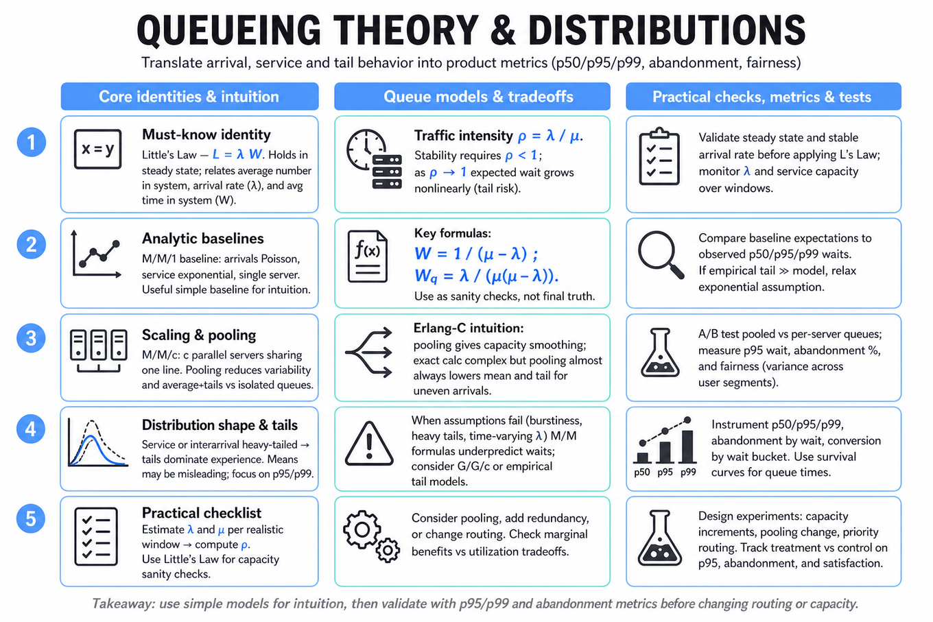
• Little’s Law is the must-recall queueing identity: $L = \lambda W$ where $L$ is average number in system, $\lambda$ is average arrival rate, and $W$ is average time in system. It is broadly applicable under steady state, regardless of arrival or service-time distribution, as long as the system is stable.

• Traffic intensity or utilization is usually $\rho = \lambda / \mu$ for a single-server queue with arrival rate $\lambda$ and service rate $\mu$. Stability requires $\rho < 1$; as $\rho \to 1$, expected wait grows nonlinearly, so “only 90% utilized” can still mean painful tail waits.

• In an M/M/1 queue, arrivals are Poisson, service times are exponential, and there is one server. Key formulas include $W = 1/(\mu-\lambda)$ for time in system and $W_q = \lambda/(\mu(\mu-\lambda))$ for time waiting before service. These are useful baselines, not universal truths.

• In an M/M/c queue, there are $c$ parallel servers sharing one line. Exact Erlang-C calculations can be complex, but the practical intuition is clear: pooling capacity reduces variability and usually lowers average and tail wait compared with separate isolated queues, especially when arrivals are uneven.

• Single queue versus multiple queues is a fairness and variance tradeoff. A single pooled queue generally minimizes expected wait and reduces “wrong line” risk; multiple queues may improve specialization, perceived autonomy, or routing quality if different servers have different skill or service-time distributions.

• Service-time variability matters as much as mean service time. With a G/G/1 queue, Kingman’s approximation says $W_q \approx \frac{\rho}{1-\rho} \cdot \frac{c_a^2+c_s^2}{2} \cdot E[S]$ where $c_a^2$ and $c_s^2$ are squared coefficients of variation for arrivals and service. High variability inflates waits.

• Poisson processes model independent random arrivals with rate $\lambda$, where counts follow $N(t)\sim \text{Poisson}(\lambda t)$ and interarrival times follow $\text{Exponential}(\lambda)$. They are a starting point for arrivals, but real product traffic often has time-of-day seasonality, bursts, and correlated behavior.

• Exponential distributions are memoryless: $P(X>s+t\mid X>s)=P(X>t)$. This property makes Markov-chain derivations tractable, but it is often unrealistic for human task times, which may be lognormal, gamma, Weibull, or heavy-tailed depending on the workflow.

• Waiting for patterns in Bernoulli trials is commonly solved with recurrence equations or a small Markov chain. For example, the expected number of fair coin flips until two consecutive heads is $6$, not $4$, because partial progress can be lost after a tail.

• Mean, median, and mode separate sharply under skewed distributions. For right-skewed data such as response times, income, follower counts, or session lengths, typically mean $>$ median $>$ mode. Reporting only the mean can hide the experience of most users or obscure tail-risk segments.

• Heavy-tailed and power-law distributions appear in network degree, creator impressions, job applications per posting, and engagement counts. A small number of members or entities can dominate totals, so robust summaries like median, trimmed mean, quantiles, log-scale plots, and segment-level metrics are often more informative.

• L1 versus L2 estimators connect distributional assumptions to modeling choices. Minimizing squared error targets the conditional mean and is sensitive to outliers; minimizing absolute error targets the conditional median and is more robust for skewed or heavy-tailed outcomes like wait time or message response delay.

Worked example

For Single Queue vs Multiple Queues — Service Design, a strong candidate should start by clarifying the unit of analysis: are people, tickets, recommendations, or tasks arriving; are servers identical; and is the goal to minimize average wait, p95 wait, abandonment, fairness, or business value? I would declare a simple baseline assumption first: arrivals are approximately random with rate $\lambda$, service capacity is $\mu$ per server, and the system is stable, then immediately note that I would validate those assumptions empirically.

The answer can be organized around four pillars. First, use capacity pooling: a single queue feeding multiple identical servers usually lowers wait because idle capacity is shared. Second, address variance and fairness: multiple queues create “line lottery” effects, where two users arriving at similar times may experience very different waits. Third, account for heterogeneity: if servers have specialized skills or tasks differ materially in service time, routing may outperform a pure single queue. Fourth, propose measurement: compare p50, p95, abandonment, reassignments, satisfaction, and downstream conversion across randomized or quasi-experimental exposure.

One explicit tradeoff to flag is that minimizing average wait may not maximize perceived fairness or task quality. For example, routing high-complexity cases to experts may increase average wait slightly but improve resolution quality and long-term retention. I would close by saying that, with more time, I would segment by arrival burstiness, task complexity, and priority class, then simulate counterfactual policies using observed arrival and service-time distributions before recommending an online experiment.

A second angle

For Derive expectation for two consecutive heads, the same stochastic reasoning appears in a cleaner mathematical form. Instead of comparing service designs, you define states: no current head streak, one head in a row, and absorbing success after two heads. Let $E_0$ be expected flips from no streak and $E_1$ from one head; then write recurrences based on the next flip rather than trying to enumerate all possible sequences. The key transfer is recognizing that state captures relevant history, just as queue length, server availability, or current workload captures relevant history in service systems. The constraint is different: here the interviewer wants exact derivation and comfort with probability, while the service-design version rewards approximation, assumptions, and empirical validation.

Common pitfalls

Pitfall: Treating all queues as if they are M/M/1.

A tempting answer is to memorize $W=1/(\mu-\lambda)$ and apply it everywhere. That misses pooled servers, priority routing, non-exponential service times, bursty arrivals, and user abandonment. A better answer uses M/M/1 as a baseline, then states which real-world features would bias the estimate.

Pitfall: Optimizing the mean while ignoring tail behavior.

For user experience, average wait can improve while p95 or p99 gets worse for important segments. This is especially dangerous with skewed service times or heavy users. Strong candidates discuss mean, median, variance, and tail percentiles, then tie the choice of metric to the product objective.

Pitfall: Jumping to formulas without framing assumptions.

Interviewers often care less about algebra speed than whether you know when the algebra applies. Before deriving, say what is random, what is independent, whether the process is stationary, and what metric you are optimizing. That communication makes even an approximate answer sound scientifically grounded.

Connections

Interviewers may pivot from queueing into survival analysis for time-to-response or time-to-abandonment, A/B testing for service-policy changes, causal inference when routing is not randomized, or ranking/recommender evaluation when queues represent candidate pools competing for limited attention. They may also connect distribution shape to robust metrics, anomaly diagnosis, or model loss functions such as absolute versus squared error.

Further reading

• Sheldon Ross, Introduction to Probability Models — strong coverage of Poisson processes, Markov chains, renewal processes, and queueing basics.

• Mor Harchol-Balter, Performance Modeling and Design of Computer Systems — practical intuition for queues, variability, pooling, and tail behavior.

• William Feller, An Introduction to Probability Theory and Its Applications — classic reference for recurrence reasoning and pattern waiting-time problems.