Uber Data Scientist Interview Prep Guide

Technical Screen

Analytics & Experimentation

• ETA Evaluation And Prediction — covered in depth under Onsite below.

• A/B Testing And Experiment Design — covered in depth under Onsite below.

• Switchback Experiments And Marketplace Interference — covered in depth under Onsite below.

• Product Metrics And Marketplace Diagnostics — covered in depth under Onsite below.

Statistics & Math

• Power Analysis And Statistical Inference — covered in depth under Onsite below.

• Causal Inference And Identification — covered in depth under Onsite below.

Data Manipulation (SQL/Python)

What's being tested

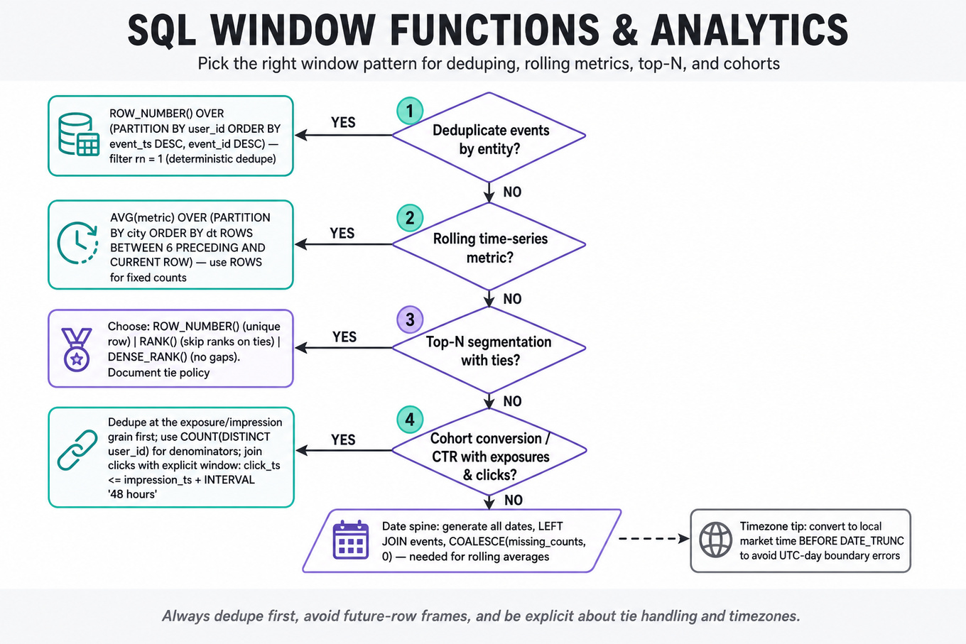
Tests SQL windowing for product analytics: cohort metrics, rolling time-series summaries, deduped event funnels, top-N segmentation, and experiment readouts. Uber DS interviews probe whether you can turn messy trip/user/event tables into defensible metrics without double-counting users, leaking future data, or mishandling time boundaries.

Patterns & templates

• Last/first event per entity — ROW_NUMBER() OVER (PARTITION BY user_id ORDER BY event_ts DESC, event_id DESC); filter rn = 1 for deterministic deduping.

• Rolling metrics — AVG(metric) OVER (PARTITION BY city ORDER BY dt ROWS BETWEEN 6 PRECEDING AND CURRENT ROW); use ROWS for fixed row counts.

• Rolling percentiles — PERCENTILE_CONT(0.5) WITHIN GROUP (ORDER BY eta) over a 7-day frame; check warehouse support and NULL handling.

• Cohort conversion / CTR — define denominator once, dedupe exposures/clicks with COUNT(DISTINCT user_id), and join within explicit windows like click_ts <= impression_ts + INTERVAL '48 hours'.

• Top-N ranking — RANK, DENSE_RANK, or ROW_NUMBER depending on tie behavior; always state whether tied promos/drivers/users should both appear.

• Date spine joins — generate all dates, left join events, COALESCE missing counts to zero; needed for rolling averages and anomaly detection.

• Timezone-aware truncation — convert to local market time before DATE_TRUNC; SF January metrics should not use raw UTC day boundaries.

Common pitfalls

Pitfall: Using COUNT(*) after joining impressions to clicks inflates CTR when users click multiple times; dedupe at the user-impression grain first.

Pitfall: Computing rolling conversion with future rows, e.g. ROWS BETWEEN 3 PRECEDING AND 3 FOLLOWING, leaks information into historical metrics.

Pitfall: Treating RANK and ROW_NUMBER as interchangeable causes silent tie bugs in top-N promotion or marketplace behavior analyses.

Practice these

The practice cards below cover the canonical variants — solve all of them and time yourself.

Practice questions

Machine Learning

• Machine Learning System Design For Real-Time Decisions — covered in depth under Onsite below.

Behavioral & Leadership

• Behavioral Leadership And Stakeholder Management — covered in depth under Onsite below.

Onsite

Analytics & Experimentation

What's being tested

Uber ETA questions test whether a Data Scientist can evaluate prediction quality, design marketplace-safe experiments, and connect model changes to rider, driver, and business outcomes. Interviewers are probing for more than “lower MAE is good”: they want to see if you understand calibration, uncertainty, conversion impact, cancellation behavior, and two-sided marketplace interference. Uber cares because ETA errors directly affect rider trust, dispatch efficiency, airport throughput, driver utilization, and marketplace liquidity. Strong answers separate prediction evaluation, causal impact, and operational diagnosis instead of mixing them into one vague “ETA improved” story.

Core knowledge

• ETA labels must be defined precisely: request-to-pickup ETA, pickup-to-dropoff ETA, or total trip duration. The target should match the user-facing promise, e.g. actual wait time $= t_\text{pickup} - t_\text{request}$, with careful treatment of cancellations, reassignment, batching, and no-shows.

• Point prediction metrics capture different failure modes. MAE is interpretable in minutes, RMSE penalizes large misses, median absolute error is robust to airport/event outliers, and bias is $\text{Bias} = \frac{1}{n}\sum_i(\hat{y}_i-y_i).$ Always segment by city, time of day, weather, airport, and trip type.

• Calibration matters as much as accuracy when ETAs are shown to users. If trips predicted as 5 minutes actually average 7 minutes, the model is underestimating and may inflate conversion while increasing cancellations. Reliability curves by ETA bucket are often more useful than a single aggregate score.

• Uncertainty intervals are useful for dispatch and UX decisions. A 90% prediction interval should contain the realized arrival time about 90% of the time; evaluate with coverage, interval width, and pinball loss for quantiles. Quantile regression, conformal prediction, and calibrated residual models are common DS-level tools.

• Business metrics should separate marketplace outcomes from model-quality outcomes. Common primary metrics include request conversion, cancellation rate, completed trips, pickup delay, and rider ETA satisfaction; guardrails include driver idle time, acceptance rate, surge exposure, gross bookings, and support contacts.

• Interference violates standard A/B assumptions because one rider’s ETA treatment can affect nearby drivers and other riders. If treatment changes dispatch or demand, user-level randomization can contaminate control. Consider geo-cluster randomization, switchback experiments, or city/time-cell designs to reduce spillovers.

• Switchback experiments randomize treatment by market and time block, such as city-zone-hour cells. They are well suited to marketplace systems where supply is shared. Analyze using cluster-robust standard errors or regression with time and geography fixed effects, not naïve row-level standard errors.

• Intent-to-treat and treatment-on-treated answer different questions. ITT estimates the effect of assignment: $E[Y|Z=1]-E[Y|Z=0].$ If only some users actually see the ETA variant, TOT may require compliance adjustment or instrumental variables, with assignment as the instrument.

• Power analysis must account for clustering and serial correlation. Cluster designs inflate variance by the design effect $DEFF = 1 + (m-1)\rho,$ where $m$ is cluster size and $\rho$ is intra-cluster correlation. For switchbacks, more independent time blocks often matter more than more events within each block.

• Offline model evaluation should use temporal holdouts and realistic slices. Random row splits can leak traffic patterns because adjacent trips share road conditions, weather, and demand shocks. Prefer train on past weeks, validate on future weeks, then stress-test holidays, airports, concerts, rain, and low-supply periods.

• Causal analysis of ETA display changes must handle selection. Riders who see long ETAs may abandon before trip creation, so completed-trip-only analysis is biased. Define the funnel from app open or request screen exposure through conversion, cancellation, pickup, and completion.

• Time-series analytics often uses rolling baselines to distinguish product effects from seasonality. For example, compare 7-day median ETA by market and hour, but avoid mixing local time zones. Use DATE_TRUNC, explicit timezone conversion, and percentile functions such as percentile_cont carefully.

Worked example

For Design an ETA experiment under interference, start by clarifying the treatment: is Uber changing the displayed ETA, the prediction model behind it, or the dispatch policy using it? Then define the unit of randomization, because rider-level randomization is likely invalid if treated riders change driver allocation, pickup congestion, or demand in the same neighborhood. A strong answer would organize around four pillars: estimand, randomization design, metrics, and inference. For the estimand, say whether the goal is the effect of assigning a market-time cell to the new ETA system on conversion, cancellation, and realized wait time. For design, propose a switchback or geo-time cluster experiment, e.g. randomize zone-hour blocks within matched markets while avoiding tiny cells with unstable supply. For metrics, choose a primary metric such as completed request conversion, plus guardrails like pickup lateness, driver utilization, cancellation, and ETA calibration. For inference, use cluster-robust standard errors or a regression with geography and time fixed effects, and pre-register the analysis window and exclusion rules. A key tradeoff is that larger clusters reduce interference but lower statistical power, so you would justify cluster size using observed driver movement and historical intra-cluster correlation. Close by saying that, with more time, you would run heterogeneity analysis for airports, peak commute, low-supply periods, and new riders, because the average effect can hide trust-damaging underestimation in critical segments.

A second angle

For Compute ETA shift and conversion uplift, the same concept becomes an analytics execution problem rather than an experiment-design problem. You still need clear definitions: ETA shift could mean change in predicted ETA, actual wait time, or prediction error, and conversion uplift should be measured from the same exposure population, not only completed trips. A good answer would build a date spine, compute timezone-aware daily or hourly metrics, and compare treatment versus control using conversion-rate differences or a regression adjustment. The interviewer may care about whether you use rolling 7-day medians to reduce noise, but the DS judgment is in avoiding biased denominators and segment-mixing. The transferable principle is that ETA analysis always needs both prediction-quality metrics and behavioral outcome metrics.

Common pitfalls

Pitfall: Treating lower average ETA as automatically good.

A tempting answer is “if predicted ETA decreases and conversion increases, the model improved.” That may simply mean the product is underpromising wait times to increase clicks, causing later cancellations and lower trust. A stronger answer checks actual wait time, prediction bias, calibration by ETA bucket, cancellation after request, and support complaints.

Pitfall: Ignoring marketplace interference.

Naïve user-level A/B testing assumes one user’s treatment does not affect another user’s outcome. In ride-hailing, ETA changes can shift demand, driver assignment, airport queue behavior, and surge exposure. Say explicitly why SUTVA may fail and propose cluster, switchback, or matched-market designs with appropriate inference.

Pitfall: Over-indexing on model architecture.

For a Data Scientist interview, do not spend most of the answer on deep learning layers, map-matching internals, or serving infrastructure. It is better to explain labels, metrics, offline-vs-online gaps, calibration, experiment design, and causal interpretation. Mention model families like XGBoost, gradient-boosted trees, or quantile models only to support evaluation tradeoffs.

Connections

Interviewers can pivot from ETA evaluation into marketplace experimentation, causal inference under interference, forecast calibration, ranking/model evaluation, or funnel analytics. They may also ask for SQL/Python execution details, especially rolling medians, cohort conversion, timezone-aware aggregation, and treatment-control comparisons.

Further reading

• Trustworthy Online Controlled Experiments — Kohavi, Tang, Xu — Practical reference for experiment design, metrics, guardrails, and inference.

• Causal Inference: What If — Hernán and Robins — Clear grounding for estimands, bias, and causal assumptions.

• Conformal Prediction for Reliable Machine Learning — Balasubramanian, Ho, Vovk — Useful background for uncertainty intervals and coverage guarantees.

Practice questions

What's being tested

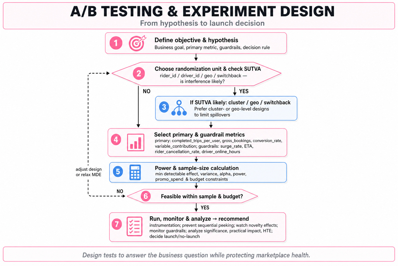
Interviewers are probing whether you can turn an ambiguous Uber product or marketplace change into a defensible causal experiment: define the hypothesis, choose the right randomization unit, select metrics, calculate power, interpret tradeoffs, and recommend launch/no-launch. Uber cares because small changes to pricing, incentives, dispatch, promos, or rider/driver experience can move gross_bookings, trips, ETA, conversion_rate, and variable_contribution in opposite directions. A strong Data Scientist does not just say “the p-value is significant”; they explain whether the result is statistically valid, practically meaningful, robust across cohorts, and safe for the marketplace. The interviewer is also testing whether you recognize interference, budget constraints, novelty effects, sequential peeking, and heterogeneous treatment effects.

Core knowledge

• Experiment objective and hypothesis should be stated before design: “Will targeted promos increase incremental gross_bookings or completed_trips at acceptable promo_spend and variable_contribution?” Separate the business goal, primary metric, guardrails, and decision rule before discussing tests.

• Randomization unit must match the causal mechanism. For rider promos, randomize at rider_id; for driver incentives, randomize at driver_id; for marketplace changes affecting matching, pricing, or supply-demand balance, consider geo-level or switchback designs because rider-level treatment can spill over to untreated users.

• Stable Unit Treatment Value Assumption (SUTVA) is often fragile at Uber. If treated riders increase demand, untreated riders may face longer ETA or higher surge. If treated drivers supply more hours, control riders benefit. Call out interference explicitly and propose cluster, geo, or time-based designs when needed.

• Primary metrics should measure incremental value, not just engagement. Common choices include completed_trips_per_user, conversion_rate, gross_bookings, net_revenue, variable_contribution, promo_spend_per_incremental_trip, cancellation_rate, ETA, and driver_online_hours. Avoid optimizing trips if the treatment destroys margin.

• Guardrail metrics protect marketplace health and user experience. For Uber, relevant guardrails include surge_rate, request_to_accept_rate, driver_utilization, rider_cancellation_rate, driver_cancellation_rate, support_contact_rate, fraud_rate, and latency-sensitive product metrics where applicable. Guardrails usually do not all need to be powered like the primary metric, but large adverse movements matter.

• Power and sample size depend on minimum detectable effect, baseline variance, alpha, and power. For a two-sample comparison of means with equal allocation:
  $n \approx \frac{2(z_{1-\alpha/2}+z_{1-\beta})^2\sigma^2}{\delta^2}$
  where $\delta$ is the minimum detectable effect. For proportions, use $\sigma^2 \approx p(1-p)$; for heavy-tailed spend metrics, consider winsorization, log transforms, or bootstrap confidence intervals.

• Z-test vs T-test depends on whether population variance is known and sample size. In large Uber experiments with thousands or millions of users, Z-tests and T-tests converge by the Central Limit Theorem. For smaller samples, unknown variance, or cluster-level analyses with few geos, use T-tests, Welch’s correction, or randomization inference.

• Variance reduction can materially improve power. CUPED uses pre-experiment covariates to reduce metric variance:
  $Y_{cuped}=Y-\theta(X-\bar X), \quad \theta=\frac{Cov(Y,X)}{Var(X)}$
  Pre-period trips, gross_bookings, or session_count can help, as long as the covariate is not affected by treatment.

• Sequential testing must control false positives. Repeatedly checking p-values and stopping when significant inflates Type I error. If business constraints require interim reads, propose alpha-spending functions, group sequential boundaries, always-valid p-values, or a pre-specified monitoring plan rather than informal peeking.

• Segmentation and heterogeneity are essential but dangerous. Analyze cohorts such as new vs existing riders, high-frequency vs low-frequency users, city tier, airport vs non-airport trips, and driver tenure. Treat segment cuts as exploratory unless pre-registered or corrected with methods like Bonferroni, Benjamini-Hochberg false discovery rate, or hierarchical modeling.

• Launch recommendations should integrate statistical and practical significance. A result can be statistically significant but not worth launching if the lift is tiny, operationally expensive, or hurts variable_contribution. Conversely, a directionally positive but underpowered result may justify extending the test, narrowing to promising cohorts, or redesigning the experiment.

• Diagnostics before interpretation should include sample ratio mismatch, pre-treatment balance, logging completeness from queried event tables, exposure validity, outliers, and novelty or day-of-week effects. A clean read requires asking whether treatment was actually delivered, eligibility was applied consistently, and the analysis window matches the user journey.

Worked example

For Analyze T2 Results and Recommend Launch Strategy, a strong candidate would start by clarifying what “T2” changed, who was eligible, the unit of randomization, the experiment duration, and the intended business objective: growth, margin, retention, or marketplace balance. They would state assumptions: “I’ll treat this as a randomized rider-level or market-level experiment and evaluate both gross_bookings and variable_contribution, with guardrails on cancellations, ETA, and supply health.” The answer should be organized around four pillars: validity of the experiment, primary and secondary metric readout, segment-level heterogeneity, and launch recommendation.

The candidate should first check whether treatment/control assignment was balanced, exposure was correct, and there was no sample ratio mismatch. Next, they would compare treatment effects with confidence intervals, not just p-values: “If gross_bookings rose 3% but variable_contribution fell 8%, I would not call this a clean win.” Then they would inspect whether the result is concentrated in strategic cohorts, such as new riders, high-LTV users, or constrained cities, while being careful not to overfit post hoc segments. One explicit tradeoff to flag is whether Uber should accept lower short-term margin for higher long-term retention; the right answer depends on measured downstream value or a credible proxy like repeat trips after the promo window. A strong close would be: “I would launch only to cohorts where incremental contribution or retention-adjusted value is positive, keep guardrails monitored, and if I had more time I’d estimate longer-term lift and run a holdout to measure promo habituation.”

A second angle

For Design an A/B test for promo-targeting models, the same experimentation principles apply, but the core challenge is evaluating an allocation policy rather than a simple product toggle. The candidate should clarify whether the new model changes who receives promos, promo amounts, or both, because that affects randomization, budget, and interpretation. A clean design might randomize eligible riders into current targeting versus new targeting, with fixed budget caps and metrics like incremental completed_trips, gross_bookings, promo_spend, and variable_contribution. The key constraint is that model scores are not causal by themselves; the experiment must estimate incremental lift versus the existing policy. The candidate should also discuss throttling or staged rollout from an analysis perspective: start with a limited eligible population, monitor guardrails, and avoid changing budgets mid-test in a way that confounds treatment effects.

Common pitfalls

Pitfall: Treating statistical significance as the launch decision.

A weak answer says, “p < 0.05, so launch.” A better answer asks whether the confidence interval excludes economically irrelevant effects, whether variable_contribution or promo_spend worsened, and whether the effect holds in the populations Uber actually wants to scale to.

Pitfall: Ignoring marketplace interference.

Randomizing individual riders is tempting because it is simple and powerful, but it may be invalid if the treatment affects driver supply, surge, or matching outcomes for other users. A stronger candidate says when user-level randomization is acceptable and when to use geo-level, cluster, or switchback designs.

Pitfall: Listing metrics without a decision framework.

Candidates often name ten metrics but never say which one decides success. Land better by declaring one primary metric, a small set of guardrails, a pre-specified analysis window, and a launch rule such as “launch if variable_contribution is non-negative and completed_trips increases by at least the MDE without guardrail regressions.”

Connections

Interviewers may pivot from here into causal inference, especially difference-in-differences, instrumental variables, or synthetic controls when randomized tests are infeasible. They may also ask about metric design, marketplace dynamics, ranking/model evaluation, or long-term treatment effects such as retention, cannibalization, and promo fatigue.

Further reading

• Trustworthy Online Controlled Experiments — Kohavi, Tang, and Xu’s practical reference on experiment design, metrics, pitfalls, and organizational decision-making.

• Controlled experiments on the web: survey and practical guide — Foundational paper by Kohavi et al. covering online A/B testing issues like ramp-up, metrics, and validity.

• Improving the Sensitivity of Online Controlled Experiments by Utilizing Pre-Experiment Data — The original CUPED paper, useful for explaining variance reduction in large-scale experiments.

Practice questions

What's being tested

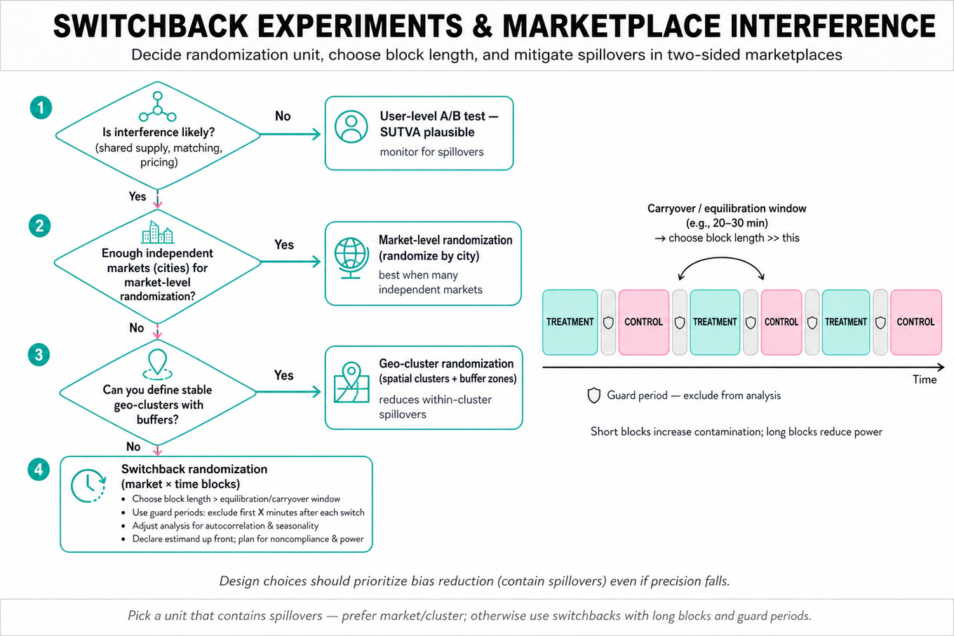
Interviewers are probing whether you can design and analyze causal experiments in two-sided marketplaces where one user’s treatment can affect another user’s outcome. At Uber, rider-facing, driver-facing, pricing, dispatch, and ETA changes often violate the standard no-interference assumption because drivers, riders, and trips compete for shared local supply. A strong Data Scientist must identify the right randomization unit, define a defensible estimand, choose metrics that reflect marketplace equilibrium, and explain how spillovers, carryover, noncompliance, and variance affect inference. The bar is not memorizing “use a switchback”; it is knowing when user-level A/B testing fails and how to recover credible causal evidence.

Core knowledge

• SUTVA, the stable unit treatment value assumption, fails when one unit’s outcome depends on others’ treatment assignment. In rideshare, treating some riders with lower displayed ETA or some drivers with a supply push can change matching, prices, wait times, and availability for untreated users in the same market.

• Interference should be handled by choosing units that contain the spillover. Common choices are market-level randomization, geo-cluster randomization, or switchback randomization by city-time block. User-level randomization is risky when supply, demand, dispatch, or pricing decisions interact through shared marketplace state.

• Switchback experiments randomize treatment over time within a market, for example city-hour blocks alternating between control and treatment. They are useful when market-level randomization has too few cities, but require careful handling of time trends, autocorrelation, seasonality, and carryover between adjacent blocks.

• Block length should exceed the system’s equilibration and carryover window. If a dispatch or pricing change affects driver positioning for 20–30 minutes, a 15-minute block is contaminated; a 60–120 minute block with guard periods may be more credible. Longer blocks reduce carryover but reduce sample size and power.

• Guard periods are observations excluded near treatment switches to reduce contamination. If treatment changes at 10:00 and matching dynamics stabilize by 10:10, exclude the first 10 minutes of each block from analysis. This sacrifices precision for lower bias, which is usually worth it when carryover is plausible.

• Estimands must be explicit. Intent-to-treat estimates the effect of assignment:
  $ITT = E[Y \mid Z=1] - E[Y \mid Z=0]$
  where $Z$ is randomized assignment. Treatment-on-treated or local average treatment effect may be relevant when actual exposure $D$ differs from assignment.

• Instrumental variables are useful under noncompliance when random assignment affects treatment received but not outcomes except through treatment. The Wald estimand is:
  $LATE = \frac{E[Y \mid Z=1] - E[Y \mid Z=0]}{E[D \mid Z=1] - E[D \mid Z=0]}$
  This requires relevance, exclusion restriction, monotonicity, and independence from potential outcomes.

• Cluster-robust inference is usually required because observations within a city-time block are correlated. Treating every trip as independent will understate standard errors. Analyze at the randomized unit level when possible, or use cluster-robust standard errors, block bootstrap, or randomization inference.

• Marketplace metrics should include both local and global effects. For Uber-like systems, consider completed_trips, conversion_rate, request_to_pickup_time, driver_utilization, surge_multiplier, cancellation_rate, gross_bookings, earnings_per_online_hour, and rider/driver guardrails. Avoid optimizing one side while silently harming the other.

• Variance reduction matters because switchbacks often have fewer independent units than trip-level data suggests. Use pre-period covariates, fixed effects for market and time, difference-in-differences style adjustment, or CUPED-like residualization:
  $Y_i^{adj} = Y_i - \theta(X_i - \bar X)$
  where $X_i$ is a predictive pre-treatment metric.

• Power calculations should be based on independent randomized blocks, not raw events. A city with millions of trips may still have only a few hundred usable city-hour treatment assignments. Autocorrelation, day-of-week effects, and cluster imbalance can dominate nominal sample size.

• Partial interference assumes spillovers occur within clusters but not across clusters. This can be plausible for city-level marketplaces, but weaker near geographic borders or airports. If clusters are too small, spillovers cross boundaries; if too large, the experiment may lack power.

Worked example

For “Design a switchback and choose block length,” a strong candidate would first clarify the treatment, the affected marketplace mechanism, and the expected lag: “Is this changing dispatch, pricing, driver incentives, or rider UI, and how quickly could drivers reposition or riders change request behavior?” They would state that user-level randomization is likely invalid if treated and untreated users share the same driver pool, so the natural unit is a market-time block such as city-hour or geo-hour. The answer would then be organized around four pillars: define the estimand and primary metrics, choose the randomization structure, handle carryover and seasonality, and specify the analysis plan.

A good design might randomize treatment by city and 2-hour blocks, stratified by hour-of-week so Friday evening treatment blocks are balanced against Friday evening control blocks. The candidate should explicitly mention guard periods, such as dropping the first 10–15 minutes after each switch if dispatch or driver location effects persist. For analysis, they might aggregate outcomes to block level and estimate a regression like $Y_{ct} = \alpha_c + \gamma_{hourweek} + \tau Z_{ct} + \epsilon_{ct}$ with cluster-robust or randomization-based inference. One key tradeoff is that shorter blocks increase the number of assignments and statistical power, while longer blocks reduce bias from carryover and allow the marketplace to equilibrate. A strong close would be: “If I had more time, I would run a pre-experiment using historical data to estimate autocorrelation and simulate power under different block lengths and guard-period choices.”

A second angle

For “Design an ETA experiment under interference,” the same causal issue appears, but the treatment is more likely rider-facing and may involve partial compliance or perception effects. If only some riders see a modified ETA, user-level randomization can still contaminate outcomes because treated riders may take trips that would otherwise be served by untreated riders. The candidate should consider market-time randomization or at least geo-cluster randomization and define whether the estimand is the effect of assigned ETA display or the effect of actually changing rider beliefs and behavior. Metrics would include request_conversion, rider_cancellation_rate, actual_wait_time, pickup_distance, and driver-side guardrails such as utilization. If assignment changes displayed ETA but not every rider notices or acts on it, instrumental variables can be introduced to estimate the effect among compliers, while still reporting the policy-relevant ITT.

Common pitfalls

Pitfall: Treating trips or users as independent when the randomized unit is market-time.

A tempting but wrong analysis is to run a trip-level t-test over millions of observations and claim extremely tight confidence intervals. That ignores within-block correlation and marketplace spillovers. A better answer aggregates to randomized units or uses cluster-robust/randomization-based inference aligned with the assignment mechanism.

Pitfall: Saying “randomize by city” without discussing power or heterogeneity.

City-level randomization reduces interference but may leave only a small number of independent units, and cities differ massively in demand patterns, regulation, airport share, and driver behavior. A stronger candidate explains the tradeoff between contamination and power, then proposes stratification, switchbacks, fixed effects, or matched markets as appropriate.

Pitfall: Jumping to instrumental variables without defending assumptions.

For IV, it is not enough to say assignment is random. You must argue that assignment strongly changes treatment received, affects outcomes only through that treatment, and does not create direct behavioral or marketplace effects outside the exposure channel. In Uber settings, exclusion restriction is often the hardest assumption because assignment can alter supply-demand balance for everyone in the cluster.

Connections

Interviewers may pivot from here to difference-in-differences, cluster randomized trials, power analysis, CUPED variance reduction, or network experiments. They may also ask how the same reasoning applies to driver incentives, surge pricing, dispatch algorithms, push notifications, ranking, or recommender evaluation in a marketplace.

Further reading

• Kohavi, Tang, and Xu, Trustworthy Online Controlled Experiments — Practical treatment of online experimentation, metrics, variance, and common failure modes.

• Hudgens and Halloran, “Toward Causal Inference With Interference” — Seminal paper on causal estimands when one unit’s treatment affects another unit’s outcome.

• Imbens and Rubin, Causal Inference for Statistics, Social, and Biomedical Sciences — Rigorous foundation for potential outcomes, instrumental variables, and randomized experiment analysis.

Practice questions

What's being tested

Interviewers are probing whether you can translate ambiguous marketplace symptoms into measurable hypotheses, validate whether the metric movement is real, and design a credible analysis or experiment to estimate impact. For Uber, small changes in ETA, price, driver supply, rider demand, cancellation, or safety metrics can interact through a two-sided marketplace, so a Data Scientist must reason beyond a single conversion funnel. Strong answers show fluency in metric design, causal inference, segmentation, experiment design, and diagnostic sequencing: first confirm the signal, then isolate where and for whom it changed, then test mechanisms. The interviewer is also looking for judgment: when to use randomized experiments, when observational methods are acceptable, and how to avoid optimizing a local metric while harming marketplace health.

Core knowledge

• Metric validation comes before explanation. Confirm numerator, denominator, time window, eligibility rules, deduping, and logging coverage for metrics like accidents_per_million_trips, completed_trips, request_to_pickup_eta, or rider_cancellation_rate. A spike can be a real product issue, a denominator collapse, or a reporting/classification change.

• Rate metrics should be decomposed as $\text{rate}=\frac{\text{events}}{\text{exposure}}.$ For accident rate, exposure could be trips, miles, hours_online, or active_drivers; each answers a different causal question. Always inspect numerator and denominator separately before interpreting the ratio.

• Marketplace balance requires supply and demand views together. Key diagnostics include requests, completed_trips, driver_hours, acceptance_rate, surge_multiplier, dispatch_eta, pickup_eta, cancellation_rate, and utilization. A rider-side decline can originate from fewer riders, higher prices, worse ETAs, lower driver supply, or degraded matching efficiency.

• Funnel analysis should identify the first point of degradation: app open → fare estimate → request → match → pickup → trip completion → repeat. Segment by city, hour-of-week, rider tenure, product type, price sensitivity, and supply conditions. Avoid averaging across markets because Simpson’s paradox is common in global marketplace data.

• Cohort analysis separates acquisition, activation, retention, and frequency. For ride declines, compare fixed rider cohorts by signup week or first-trip month and track week_1_retention, rides_per_active_rider, and reactivation. This distinguishes “fewer new riders” from “existing riders riding less.”

• Causal inference starts with a target estimand, such as average treatment effect: $ATE = E[Y(1)-Y(0)].$ If randomization is possible, prefer an A/B test; if not, consider difference-in-differences, synthetic control, propensity score weighting, or matched market analysis, while stating assumptions like parallel trends and no unmeasured confounding.

• Experiment design in a marketplace must choose the correct randomization unit. Rider-level experiments are good for promotions or subscriptions, but pricing, dispatch, and ETA changes can create interference through shared driver supply. Market-level, geo-level, or switchback designs are often more appropriate when treatments affect equilibrium.

• Power analysis should account for skew, clustering, and rare events. For binary outcomes, a rough sample size per arm is $n \approx \frac{2(z_{\alpha/2}+z_\beta)^2p(1-p)}{\delta^2}.$ For rare safety events or accident rates, simple A/B tests may be underpowered; use longer windows, exposure modeling, Bayesian shrinkage, or hierarchical models.

• Guardrail metrics prevent local optimization. Lowering ETA may improve conversion but hurt driver_utilization, pickup_distance, cancellation_rate, surge, or long-run retention. Ad effectiveness may lift signups but fail on incremental_trips, gross_bookings, contribution margin, or payback period.

• Composite indices need transparent construction. A Market Balance Index might combine standardized ETA, surge, cancellation_rate, driver_utilization, and completion_rate: $MBI = \sum_i w_i z_i.$ Weights should reflect business relevance, stability, and interpretability; validate against downstream outcomes like retention and completed trips.

• Survival and hazard models are useful when timing matters. For rider wait experience, model probability of cancellation as a function of elapsed wait time: $h(t)=P(T=t \mid T \ge t).$ This can reveal whether a 1-minute ETA increase is harmless early but sharply increases cancellation after a threshold.

• Heterogeneous treatment effects are expected. Effects differ by market density, rider tenure, product tier, commute versus leisure trips, weather, airport trips, and time of day. Pre-specify the most important segments; avoid fishing across hundreds of cuts without correction or a clear exploratory label.

Worked example

For Analyze the Accident-Rate Spike, a strong candidate should first clarify the metric: “Is this accidents per completed trip, per mile, per active driver hour, or per reported incident, and did the reporting policy change?” They would also ask about the time window, affected geographies, product types, and whether the spike appears in both raw counts and normalized rates. The answer can be organized into four pillars: validate the data signal, decompose numerator versus denominator, segment to localize the change, and evaluate causal hypotheses.

The candidate might start by plotting accidents, completed_trips, miles_driven, and accidents_per_million_miles over time, with confidence intervals because accidents are rare and noisy. Then they would segment by city, hour, weather, road type proxy, driver tenure, vehicle type, and trip distance to see whether the spike is broad-based or concentrated. Next, they would compare against external context such as holidays, storms, regulatory changes, or changes in incident reporting, while staying at the analytics layer rather than proposing data pipeline architecture. A key tradeoff is choosing the exposure denominator: per trip can falsely suggest risk increased if average trip distance rose; per mile may better reflect driving exposure, but per pickup or per hour might matter for marketplace operations. They would close by saying: if more time were available, they would build a monitored safety risk model with market-level baselines, anomaly thresholds, and pre-specified escalation criteria.

A second angle

For How to evaluate lowering ETA?, the same diagnostic skill applies, but the problem shifts from explaining a metric movement to estimating the impact of an intervention. The first step is defining whether “lowering ETA” means showing a lower displayed estimate, improving actual pickup time, changing dispatch radius, or repositioning supply, because each has different causal mechanisms. The primary metrics might be request_conversion_rate, completed_trips, actual pickup_wait_time, and rider_retention, with guardrails on driver_pickup_distance, driver_earnings_per_hour, cancellation_rate, and marketplace_balance. Because dispatch changes affect shared supply, a simple rider-level A/B test may violate independence; a switchback or geo experiment can better estimate marketplace effects. The core idea is identical: define the estimand, protect against confounding, and read both rider and driver-side metrics.

Common pitfalls

Pitfall: Treating every movement as a product effect before validating the metric.

A tempting answer is “accidents spiked because driver quality got worse” or “rides declined because users dislike the new price.” A stronger answer first checks whether the numerator, denominator, logging definitions, reporting rules, or mix of markets changed, then moves into behavioral explanations.

Pitfall: Optimizing one side of the marketplace in isolation.

For example, saying “lower ETA is successful if rider conversion increases” misses driver pickup burden, supply utilization, and market-wide interference. A better answer defines a primary rider outcome plus driver and marketplace guardrails, and explains why the randomization unit must match the treatment’s spillover pattern.

Pitfall: Listing metrics without a decision framework.

Interviewers are not impressed by a long inventory of DAU, conversion, retention, revenue, and NPS unless you explain which metric is primary, which are diagnostics, and what decision each would support. State the hierarchy: north-star outcome, input metrics, guardrails, segments, and the launch/no-launch threshold.

Connections

Interviewers may pivot into switchback experiments, difference-in-differences, marketplace pricing and surge diagnostics, ranking or dispatch model evaluation, or incrementality measurement for paid marketing. Be ready to discuss interference, clustered standard errors, sequential monitoring, and how online experiment results can diverge from offline model metrics.

Further reading

• Trustworthy Online Controlled Experiments — Practical reference on experiment design, guardrails, novelty effects, and interpretation at scale.

• Causal Inference: The Mixtape — Clear treatment of difference-in-differences, synthetic control, matching, and regression discontinuity.

• Marketplace Experimentation — Useful industry framing for interference, switchbacks, and two-sided marketplace experiment design.

Practice questions

Statistics & Math

What's being tested

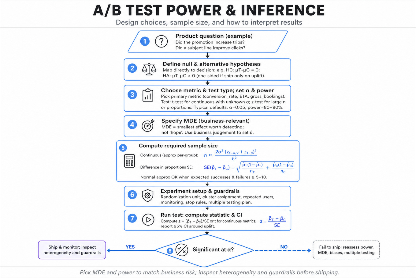
Interviewers are probing whether you can design and interpret A/B tests as a Data Scientist, not just plug numbers into a calculator. You need to translate product questions like “did this promotion increase trips?” or “did this subject line improve clicks?” into hypotheses, metrics, power assumptions, test statistics, and decision rules. Uber cares because small changes to conversion_rate, ETA, gross_bookings, driver_accept_rate, or cancellation_rate can have large marketplace effects, and bad inference can ship harmful changes or reject valuable ones. The strongest answers show statistical correctness, business judgment, and awareness of messy experimental realities like skewed revenue, repeated users, cluster assignment, guardrails, and multiple testing.

Core knowledge

• Null and alternative hypotheses should map directly to the product decision. For a promotion test, $H_0: \mu_T - \mu_C = 0$ and $H_A: \mu_T - \mu_C > 0$ may fit if you only ship on uplift; use two-sided tests when either harm or benefit matters.

• Type I error, Type II error, and power are the foundation. Significance level $\alpha$ is the false-positive rate, $\beta$ is the false-negative rate, and power is $1-\beta$. Common defaults are $\alpha=0.05$ and power $=80\%$ or $90\%$, but the right choice depends on launch risk and opportunity cost.

• Minimum detectable effect (MDE) is the smallest effect worth detecting, not the effect you hope to see. For a two-arm test with equal allocation and continuous outcomes, an approximate per-group sample size is:
  $n \approx \frac{2\sigma^2(z_{1-\alpha/2}+z_{1-\beta})^2}{\delta^2}$
  where $\delta$ is the absolute MDE.

• For difference in proportions, such as email click_through_rate, use:
  $SE(\hat p_T-\hat p_C)=\sqrt{\frac{\hat p_T(1-\hat p_T)}{n_T}+\frac{\hat p_C(1-\hat p_C)}{n_C}}$
  and compute $z=(\hat p_T-\hat p_C)/SE$. The normal approximation is reasonable when expected successes and failures in each arm are usually at least 5–10.

• Z-tests vs t-tests depend on what is known and sample size. Use a Z-test for large-sample proportions or when variance is effectively known; use a t-test for continuous metrics with unknown variance, especially smaller samples. In large Uber experiments with thousands or millions of units, Z and t often converge, but the interviewer may test whether you know why.

• Confidence intervals are often more useful than p-values. A 95% CI for a treatment effect gives the plausible range of impact, e.g. “+0.2% to +1.1% conversion.” If the CI excludes both zero and economically trivial effects, the launch case is stronger than “p < 0.05.”

• Large p-values do not prove no effect. They mean the observed data are not sufficiently inconsistent with $H_0$ under the test assumptions. A well-calibrated answer says “we failed to reject the null,” then checks whether the test was powered for the business-relevant MDE.

• Intent-to-treat (ITT) analysis preserves randomization by analyzing users, trips, or cities according to assigned group, regardless of whether they fully received treatment. For marketplace products, ITT is usually the primary estimate because non-compliance can be correlated with user behavior and create selection bias.

• Ratio metrics like revenue_per_trip, trips_per_user, or conversion_rate need care because the numerator and denominator are random. Delta method, bootstrap, or user-level aggregation are safer than naively treating every trip as independent when users contribute multiple trips.

• Clustered observations break independence assumptions. If randomization is by city, market, driver, or user, inference should match that unit; use cluster-robust standard errors or analyze at the assignment level. Treating millions of trips as independent when only 20 cities were randomized can massively understate uncertainty.

• Variance reduction methods such as CUPED can increase power by adjusting for pre-experiment covariates. A common form is $Y_{adj}=Y-\theta(X-\bar X)$, where $X$ is a pre-period metric. It is valid when $X$ is measured before treatment and not affected by the experiment.

• Multiple testing inflates false positives across many metrics, segments, or variants. Pre-specify a primary metric and guardrails; for many planned comparisons, use methods like Bonferroni correction, Holm-Bonferroni, or Benjamini-Hochberg FDR depending on whether the priority is strict family-wise error control or discovery.

• Sequential testing requires correction if you repeatedly peek at results. Naively checking daily and stopping when $p<0.05$ increases false positives. Valid approaches include alpha-spending functions, group sequential designs, always-valid p-values, or a pre-registered fixed horizon.

• Guardrail metrics protect the marketplace from local optimization. A promotion might increase gross_bookings but hurt contribution_margin, driver_supply_hours, or cancellation_rate. A good launch rule distinguishes primary success metrics from non-negotiable guardrails.

Worked example

For “Determine Sample Size for Promotion Campaign A/B Test,” a strong candidate would start by clarifying the randomization unit, target population, primary metric, expected baseline, and business-relevant MDE. For example: “Are we randomizing riders, trips, cities, or markets? Is success incremental gross_bookings, completed_trips, conversion_rate, or profit after promo cost?” Then they would state assumptions: equal allocation, fixed-horizon test, independent user-level outcomes unless there is clustering, and a chosen $\alpha$ and power.

The answer skeleton should have four pillars: first, define hypotheses and the primary metric; second, estimate baseline variance or baseline conversion from historical data; third, compute sample size using the appropriate formula for proportions or continuous outcomes; fourth, define guardrails and an analysis plan before launch. If the metric is conversion_rate, they might use a difference-in-proportions power formula; if it is revenue_per_user, they would discuss skewness and potentially bootstrap or log-transform sensitivity checks. A specific tradeoff to flag is that a smaller MDE requires quadratically more sample: halving $\delta$ roughly quadruples required sample size. They should also mention that promotions can create interference since treated riders may affect driver availability or surge dynamics for control riders. A strong close would be: “If I had more time, I’d validate variance from a pre-period, run a power curve across plausible MDEs, and check whether cluster-level randomization is needed to reduce marketplace spillovers.”

A second angle

For “Analyze results and large p-values correctly,” the same inference machinery applies, but the emphasis shifts from planning to interpretation. The interviewer is looking for whether you avoid saying “there is no effect” when the p-value is large. A better answer separates statistical uncertainty from business relevance: “The estimate is positive but imprecise; the confidence interval includes both meaningful lift and no lift, so we may be underpowered.” This framing naturally leads to checking sample size, realized variance, treatment exposure, experiment duration, and whether the analysis used the correct unit of randomization. It also tests judgment about whether to extend the test, stop due to futility, or redesign the metric.

Common pitfalls

Pitfall: Treating p > 0.05 as proof that the treatment failed.

This is the most common analytical mistake. A large p-value may reflect a small true effect, high variance, insufficient sample size, dilution from non-compliance, or an incorrectly specified test. Say “we failed to reject the null,” then discuss the confidence interval, MDE, and realized power.

Pitfall: Choosing a metric after seeing the results.

A tempting but weak answer is “we checked many segments and found a significant increase among weekday riders, so we should launch there.” That may be p-hacking unless the segment was pre-specified or adjusted for multiple comparisons. A stronger response labels it exploratory and proposes a follow-up confirmatory test.

Pitfall: Ignoring the assignment unit and pretending all rows are independent.

If users are randomized but the dataset has one row per trip, trip-level tests can overweight frequent riders and understate standard errors. If cities are randomized, the effective sample size is closer to the number of cities than the number of trips. The better answer aggregates or uses cluster-robust inference aligned to the randomization design.

Connections

Interviewers may pivot from power analysis into causal inference, especially selection bias, non-compliance, and interference. They may also connect this to metric design, variance reduction, sequential experimentation, heterogeneous treatment effects, or ranking/model evaluation when product changes affect marketplace quality metrics beyond the primary KPI.

Further reading

• Trustworthy Online Controlled Experiments by Kohavi, Tang, and Xu — Practical treatment of online experiment design, metrics, pitfalls, and interpretation.

• CUPED: Controlled-experiment Using Pre-Experiment Data — Seminal paper on variance reduction for large-scale experiments.

• Causal Inference: The Mixtape by Scott Cunningham — Useful background on causal reasoning, identification, and interpretation beyond randomized tests.

Practice questions

What's being tested

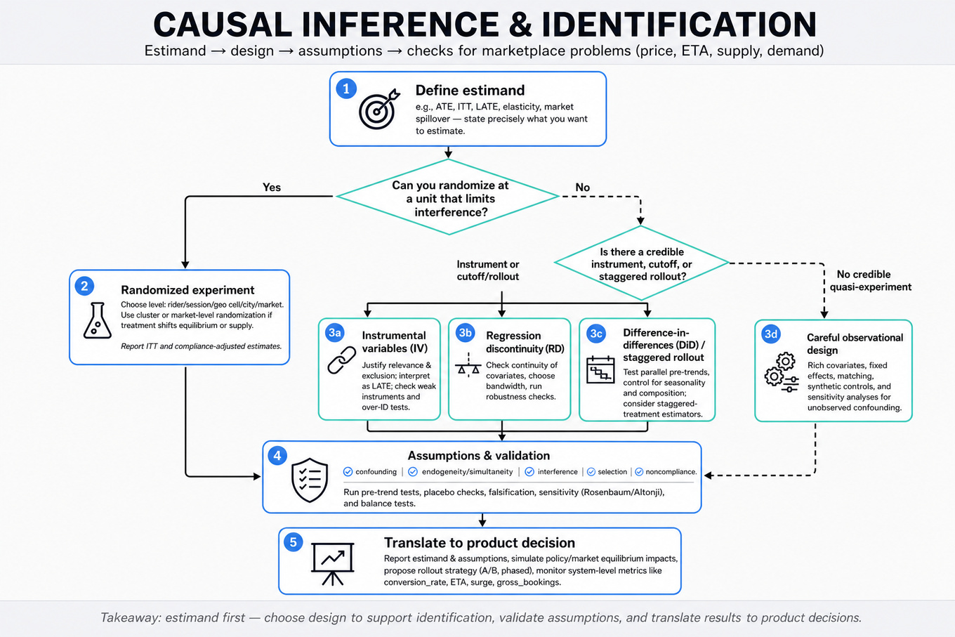
Interviewers are probing whether you can separate correlation from causation in Uber-style marketplace problems where price, ETA, demand, and supply move together. A strong Data Scientist must define the right estimand, choose an identification strategy, defend assumptions, and translate the result into a product or marketplace decision. Uber cares because metrics like conversion_rate, ETA, surge_multiplier, gross_bookings, and driver utilization are jointly determined; naive regressions can confidently recommend the wrong lever. Expect pressure on endogeneity, selection bias, interference, noncompliance, and whether your proposed estimate would actually answer the business question.

Core knowledge

• Estimand first, method second. State whether you want the average treatment effect: $ATE = E[Y(1)-Y(0)]$, intent-to-treat effect, local average treatment effect, elasticity, or market-level spillover effect. For Uber, “effect of ETA on conversion” differs from “effect of showing a lower ETA prediction.”

• Confounding occurs when treatment assignment is related to potential outcomes. Example: shorter ETA often occurs in dense areas with higher baseline conversion, so regressing conversion_rate on ETA overstates the causal benefit of reducing ETA unless geography, time, demand, rider intent, and supply are handled.

• Endogeneity and simultaneity are central in price–ETA trade-offs. Price affects demand, demand affects driver availability, driver availability affects ETA, and ETA affects conversion. A naive model like $Conversion_i = \beta_0 + \beta_1 Price_i + \beta_2 ETA_i + \epsilon_i$ usually violates $E[X_i\epsilon_i]=0$.

• Randomized experiments are the cleanest design when feasible. Randomize at the unit where interference is limited: rider, session, geo cell, city, or time block. If treatment can affect marketplace equilibrium, rider-level randomization may contaminate control via shared driver supply, so cluster or market-level randomization may be needed.

• Difference-in-differences estimates treatment effects by comparing treated and control changes over time:
  $\hat{\tau}_{DiD}=(\bar{Y}_{T,post}-\bar{Y}_{T,pre})-(\bar{Y}_{C,post}-\bar{Y}_{C,pre})$
  The key assumption is parallel trends, not equal levels. Always check pre-trends, seasonality, rollout timing, and compositional shifts.

• Instrumental variables handle unobserved confounding when you have a source of exogenous variation. A valid instrument $Z$ must satisfy relevance, $Cov(Z,X)\neq0$, exclusion, $Z$ affects $Y$ only through $X$, and independence from unobserved outcome drivers. In Uber contexts, candidates might discuss weather shocks, randomized price nudges, supply-side constraints, or dispatch rule variation, but must defend exclusions carefully.

• Two-stage least squares estimates causal effects using predicted treatment variation. First stage: $X_i=\pi_0+\pi_1Z_i+\gamma W_i+u_i$. Second stage: $Y_i=\beta_0+\beta_1\hat{X}_i+\delta W_i+\epsilon_i$. Report first-stage strength, often using an F-statistic rule of thumb above 10, and interpret $\beta_1$ as a LATE for compliers.

• Elasticity estimation often uses log-log models: $\log(Q_i)=\alpha+\beta\log(P_i)+\gamma W_i+\epsilon_i$, where $\beta$ is price elasticity. But if price is dynamically set based on demand, the model identifies association unless price variation is randomized or instrumented.

• Interference violates SUTVA when one user’s treatment affects another user’s outcome. In rideshare, changing ETAs or prices for some riders changes driver availability, wait times, and conversion for others. Handle with cluster randomization, exposure mappings, market-level aggregates, or estimands like direct effect, spillover effect, and total effect.

• Noncompliance means assignment differs from actual exposure. For example, a rider assigned to see a new ETA treatment may not open the app, or a city assigned to a pricing change may only partially roll it out. Estimate ITT for policy impact; use IV/Wald estimators for complier effects: $\frac{E[Y|Z=1]-E[Y|Z=0]}{E[D|Z=1]-E[D|Z=0]}$.

• Diagnostics matter as much as estimation. For experiments, check balance, sample ratio mismatch, guardrail metrics, and heterogeneous treatment effects. For DiD, inspect pre-period event-study coefficients. For IV, test instrument strength and argue exclusion qualitatively; no statistical test can fully prove exclusion.

• Aggregation level changes interpretation. Session-level data supports individual conversion models, while geo-hour or city-week panels capture marketplace equilibrium. With millions of sessions, standard errors can still be wrong if treatment varies by market; use cluster-robust standard errors at the assignment or shock level, not just row-level n.

Worked example

For “Estimate price–ETA trade-offs causally”, a strong candidate would start by clarifying the decision: are we estimating how much conversion changes if Uber increases price holding ETA fixed, decreases ETA holding price fixed, or changes a dispatch/pricing policy that moves both? They would define the outcome, likely conversion_rate, completed_trips, or contribution margin, and specify whether the unit is request, session, geo-hour, or market-day. The answer should be organized around four pillars: first, explain why naive regression is biased because price, ETA, demand, and supply are jointly determined; second, propose a preferred experiment if feasible, such as randomized price or ETA-display perturbations with guardrails; third, offer an observational fallback using IV or DiD; fourth, discuss diagnostics and interpretation.

A candidate might propose an IV where random price nudges or algorithmic threshold discontinuities shift price but are plausibly unrelated to rider intent except through price. They should immediately flag the exclusion restriction: if the same mechanism also changes ETA, the instrument may not isolate price unless ETA is modeled as a separate endogenous variable or the estimand is the joint policy effect. The 2SLS skeleton would use first-stage models for price and/or ETA, then a second-stage conversion model with market-time controls and clustered standard errors. A key tradeoff is between internal validity and external validity: a small randomized nudge gives clean identification around current prices but may not extrapolate to large surge changes. To close, they could say: “If I had more time, I’d estimate heterogeneous elasticities by city, rider segment, and trip purpose, and compare short-run conversion effects with marketplace equilibrium effects on driver supply.”

A second angle

For “Evaluate ETA Impact on Conversion”, the same causal logic applies, but the treatment is more likely a service quality variable than a direct product knob. The tempting analysis is to bucket sessions by observed ETA and compare conversion, but that confounds ETA with density, weather, airport trips, rider urgency, and driver supply. A stronger framing distinguishes the effect of actual ETA reduction from the effect of displaying a different ETA prediction. If experimenting on actual ETA is hard because dispatch changes affect the whole market, the candidate should discuss cluster randomization or quasi-experimental variation in supply shocks. The best answer also notes interference: reducing ETA for treated riders may increase ETA for untreated riders competing for the same drivers.

Common pitfalls

Pitfall: Treating controls as a cure-all.

A common analytical mistake is saying “I’ll control for city, time, and rider features, then regress conversion on ETA.” That may reduce observed confounding, but it does not solve unobserved intent, simultaneity, or marketplace equilibrium effects. A better answer explicitly states the identifying assumption and why it may or may not be believable.

Pitfall: Not naming the estimand.

Candidates often jump into 2SLS, DiD, or experimentation without saying what effect they want. Interviewers will push: is this the effect on riders exposed to treatment, all riders in the market, complisers, or the total marketplace effect including spillovers? Start with the estimand, then choose the design.

Pitfall: Ignoring interference in a two-sided marketplace.

A rider-level A/B test sounds clean but can fail when treated and control users share the same driver pool. If the treatment changes driver allocation, wait times, or surge, control outcomes are contaminated. A stronger answer proposes geo-level randomization, switchback experiments, or explicit spillover estimands.

Connections

Interviewers may pivot from causal identification into experiment design, especially switchback tests, cluster randomization, power, and guardrail metrics. They may also connect to metric design, marketplace dynamics, ranking/model evaluation, or segmentation, asking whether the estimated effect differs by city, time of day, rider tenure, or supply conditions.

Further reading

• Mostly Harmless Econometrics — practical treatment of IV, DiD, regression, and identification assumptions.

• Causal Inference: The Mixtape — accessible examples of DiD, IV, event studies, and modern applied causal inference.

• Design and Analysis of Switchback Experiments — useful for marketplace experiments where interference makes user-level randomization problematic.

Practice questions

What's being tested

Interviewers are probing whether you can translate a marketplace behavior, like riders abandoning after waiting too long, into a rigorous time-to-event problem rather than a simple binary classification or average-duration analysis. Uber cares because wait time, matching quality, cancellation, and price interact dynamically: a rider who has not yet abandoned after 2 minutes is a different risk population than one observed at request time. A strong Data Scientist should define the event, risk set, censoring mechanism, covariates, and evaluation metric, then connect model outputs to product or marketplace decisions. You are also expected to explain survival outputs in business language: “hazard increased 20% after ETA crossed 8 minutes” is more actionable than “model coefficient is positive.”

Core knowledge

• Survival function is $S(t)=P(T>t)$, the probability a rider has not abandoned by time $t$. Cumulative distribution is $F(t)=1-S(t)$, useful for statements like “15% of riders abandon within 3 minutes of seeing a long ETA.”

• Hazard function is $h(t)=\lim_{\Delta t\to0}\frac{P(t\le T<t+\Delta t\mid T\ge t)}{\Delta t}$. For Uber, this is the instantaneous abandonment risk among riders still waiting, not the unconditional abandonment probability.

• Right censoring occurs when the event is not observed before observation ends. A rider who gets matched, completes request, closes the app without known intent, or is still waiting at log cutoff may be censored depending on the business definition.

• Competing risks matter when multiple terminal outcomes prevent abandonment: match accepted, rider cancels, driver cancels, request expires, or trip starts. Treating every non-abandonment as ordinary censoring can bias results if those outcomes are related to abandonment risk.

• Left truncation, or delayed entry, happens when riders enter observation only after some elapsed wait time, such as sessions first logged after queue entry or only requests visible after a dispatch state. Use risk sets conditional on surviving until entry time.

• Kaplan-Meier estimator estimates $S(t)$ nonparametrically: $\hat S(t)=\prod_{t_i\le t}\left(1-\frac{d_i}{n_i}\right)$ where $d_i$ events occur among $n_i$ at risk. It is ideal for cohort curves by city, ETA bucket, surge bucket, or product surface.

• Cox proportional hazards model estimates covariate effects without specifying baseline hazard: $h(t\mid x)=h_0(t)\exp(\beta^\top x).$ A hazard ratio of $1.25$ means 25% higher instantaneous event risk, assuming proportional hazards.

• Proportional hazards assumption should be checked with Schoenfeld residuals, log-minus-log curves, or time interactions. If ETA matters strongly only after 5 minutes, include ETA × time_bucket or use a discrete-time hazard model.

• Time-varying covariates are central in Uber settings: displayed ETA, surge multiplier, driver supply nearby, app foreground status, queue position, and price estimate can change during waiting. Encode intervals as start-stop rows: (rider_id, t_start, t_end, event, covariates).

• Discrete-time survival is often practical when events are logged in seconds or minutes. Model $P(T=t\mid T\ge t,x_t)$ with logistic regression, XGBoost, or calibrated classifiers over person-period rows; works well at large scale and handles nonlinear effects.

• Model evaluation should include concordance index, time-dependent AUC, calibration by time horizon, and business lift curves. For intervention design, also report predicted abandonment probability by 1, 3, and 5 minutes, not just global discrimination.

• Market balance metrics can use survival outputs as components: wait-time abandonment hazard, probability of match within 2 minutes, price-adjusted conversion, cancellation risk, and fulfilled-trip probability. Composite indexes should normalize by market mix and avoid double-counting correlated signals.

Worked example

For Model waiting-time abandonment via survival, start by clarifying the event: “Does abandonment mean explicit rider cancellation, app exit before match, no driver accepted within timeout, or any failure before trip start?” Then declare the time origin, usually when the rider submits a request or sees the initial ETA, and define terminal states such as match, cancellation, trip start, and observation cutoff. A strong answer would organize around four pillars: event definition and censoring, exploratory survival curves, model specification, and product interpretation.

First, propose Kaplan-Meier curves by initial ETA bucket, city, time of day, and surge status to show whether abandonment risk accelerates after specific thresholds. Second, specify a Cox or discrete-time hazard model with time-varying covariates like current ETA, elapsed wait, price multiplier, driver supply, and rider history. Third, explain that right-censored riders remain informative up to their last observed time and should not be dropped. Fourth, translate outputs into actions: if hazard spikes when displayed ETA moves from 6 to 8 minutes, Uber might test better ETA messaging, incentives for nearby drivers, or earlier re-routing.

One tradeoff to flag explicitly: a Cox model is interpretable through hazard ratios, but a discrete-time XGBoost hazard can capture nonlinearities and interactions at the cost of explainability and calibration work. Close by saying that, with more time, you would test proportional hazards, perform calibration by market, and evaluate whether interventions based on the model improve cancellation, conversion, and completed trips in an experiment.

A second angle

For Define market-only rider experience metrics, the same survival logic becomes a metric-design tool rather than a standalone model. Instead of asking “when does a rider abandon?”, you define marketplace health metrics that isolate supply-demand balance: probability of getting matched within 2 minutes, survival curve of remaining unmatched, abandonment hazard after ETA changes, and cancellation risk before pickup. The “market-only” framing means you should adjust or segment away factors outside marketplace quality, such as rider intent mix, product type, weather shocks, airport rules, or price level when the goal is to measure balance. A composite Market Balance Index could combine standardized components like P(match ≤ 2m), median_wait_time, price-adjusted conversion, and abandonment hazard, but you should justify weights and show sensitivity to city, hour, and trip type. The constraint is not just statistical fit; it is metric validity, interpretability, and whether local operations teams can act on the signal.

Common pitfalls

Pitfall: Treating abandonment as a plain binary label loses timing information.

A tempting answer is “build a classifier predicting whether the rider cancels.” That ignores that a rider who waits 30 seconds and a rider who waits 9 minutes contribute very different evidence; survival modeling uses the full risk process and handles riders whose outcomes are only partially observed.

Pitfall: Calling every non-abandonment case “censored” without checking the business process.

If a rider gets matched quickly, that is not random censoring; it is a competing marketplace outcome related to driver supply and ETA. A better answer acknowledges competing risks and either models cause-specific hazards or defines the estimand carefully, such as abandonment before match.

Pitfall: Over-indexing on formulas and under-explaining product interpretation.

Interviewers do not just want $h(t)$ and $S(t)$. They want to hear how a hazard ratio, survival curve, or time-horizon probability would change marketplace decisions, metric dashboards, experiment guardrails, or rider experience interventions.

Connections

This topic often pivots into causal inference, especially whether reducing ETA causes lower abandonment versus merely correlating with higher supply. It can also connect to experiment design, marketplace metrics, calibration, ranking/model evaluation, and segmentation analysis by city, hour, rider tenure, or trip type.

Further reading

• Cox, “Regression Models and Life-Tables” (1972) — the original proportional hazards paper and foundation for hazard-ratio interpretation.

• Kleinbaum and Klein, Survival Analysis: A Self-Learning Text — practical coverage of censoring, Cox models, diagnostics, and interpretation.

• Cam Davidson-Pilon, lifelines documentation — accessible Python examples for KaplanMeierFitter, CoxPHFitter, and time-varying survival data.

Practice questions

Machine Learning

What's being tested

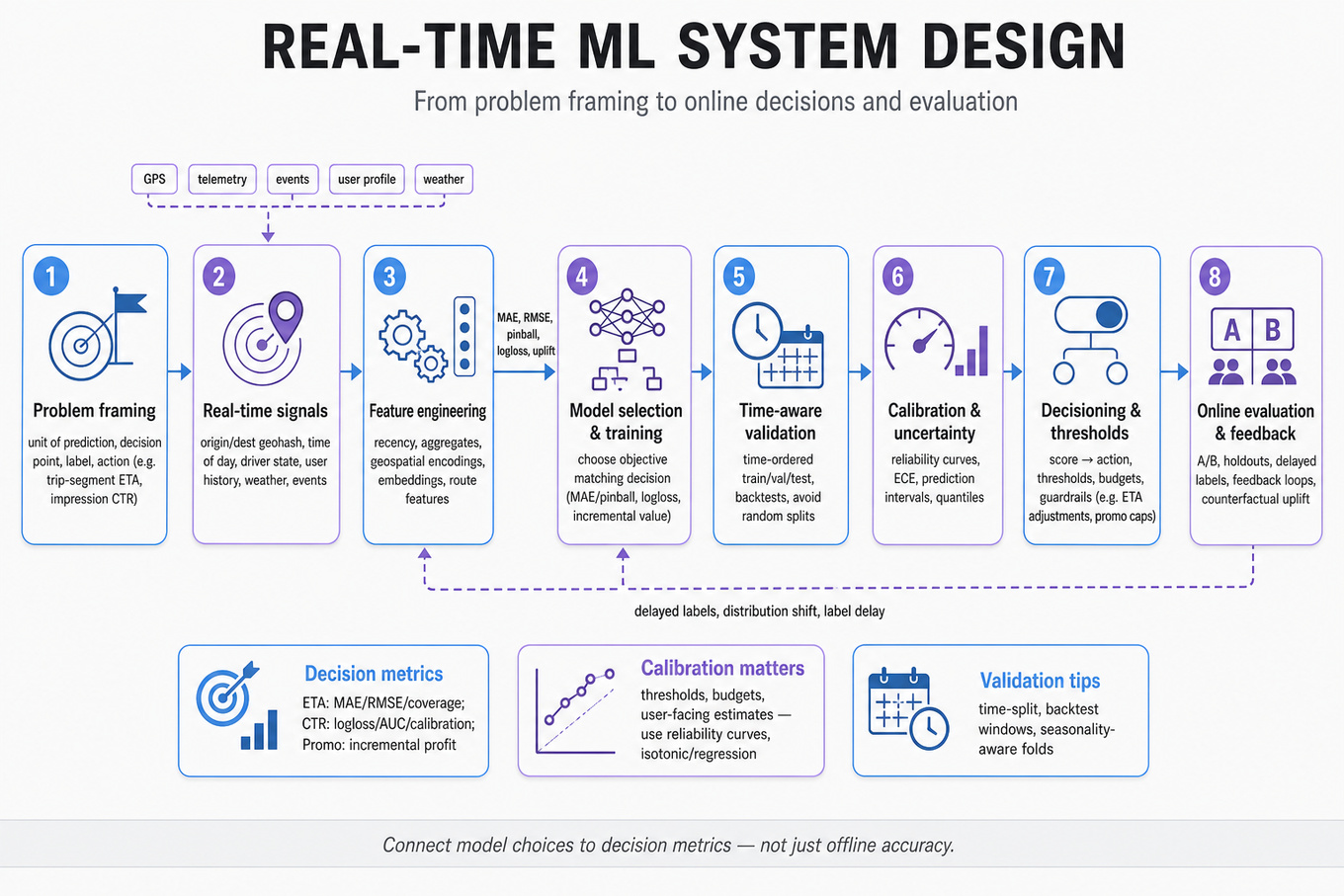
Interviewers are probing whether you can design and evaluate machine learning systems for real-time decisions from a Data Scientist’s perspective: defining the prediction target, choosing features and models, validating offline, calibrating uncertainty, and deciding whether the model improves business outcomes. Uber cares because ETA, CTR, promo targeting, and real-time clustering all directly affect marketplace efficiency, rider trust, driver utilization, and spend efficiency. The emphasis is not on building serving infrastructure; it is on whether you understand how prediction quality, calibration, bias, feedback loops, delayed labels, and online evaluation interact in a production decision system. Strong answers connect model choices to decision metrics, not just offline accuracy.

Core knowledge

• Problem framing comes first: define the unit of prediction, decision point, label, and action. For ETA, the unit may be trip segment or full trip; for CTR, an impression; for promo targeting, a user-offer decision. Misdefining the label often causes bigger errors than choosing the wrong model.

• Real-time features should be described as signal sources, not pipeline architecture. For ETA, useful signals include origin/destination geohashes, time of day, day of week, route distance, historical speeds, weather, event indicators, driver state, and recent traffic. For CTR, use user history, ad/item metadata, context, position, and recency features.

• Time-aware validation is mandatory when data distributions shift. Use train/validation/test splits ordered by time rather than random splits, especially for ETA, CTR, and promo response. A random split can leak future traffic patterns, future user behavior, or post-treatment outcomes into training.

• Loss functions should match the decision. ETA often uses MAE, RMSE, MAPE, pinball loss for quantiles, and calibration of prediction intervals. CTR uses log loss, AUC, PR-AUC, calibration error, and lift by score decile. Promo targeting should optimize incremental value: $E[\text{profit}] = p(\text{incremental conversion}) \cdot \text{margin} - \text{promo cost}.$

• Calibration matters when scores drive thresholds, budgets, or user-facing estimates. A CTR model with good AUC but poor calibration can overspend ad budget; an ETA model with biased underestimates damages rider trust. Use reliability curves, expected calibration error, isotonic regression, Platt scaling, and segment-level calibration checks.

• Uncertainty quantification is central for real-time decisions. ETA should often output intervals, not just a point estimate: “pickup in 4–6 minutes” may be better than “5 minutes.” Common approaches include quantile regression, conformal prediction, bootstrapped ensembles, and residual models by route/time segment.

• Model families should be justified by data shape and latency needs from an analytical perspective. XGBoost or LightGBM often work well for tabular CTR, ETA, and promo response baselines; neural networks can help with sparse high-cardinality features and embeddings; simple linear/logistic models remain valuable for interpretability and calibration baselines.

• Class imbalance is not solved by accuracy. CTR and promo conversion may have positive rates below 1–5%, so accuracy can be meaningless. Prefer log loss, PR-AUC, lift, recall at fixed precision, calibration by score bucket, and business metrics such as revenue per impression or cost per incremental conversion.

• Delayed feedback creates biased labels. A user may click immediately, convert hours later, or complete a ride after dispatch. Define attribution windows, account for right-censoring, and compare mature-label evaluation versus early-label proxies. For promo targeting, delayed redemption and retention effects can change the apparent winner.

• Causal evaluation is required when the model chooses interventions. Promo targeting is not just predicting who will use a coupon; it is estimating who changes behavior because of the coupon. Use randomized experiments when possible, or off-policy methods such as inverse propensity weighting: $\hat{V}_{IPS} = \frac{1}{n}\sum_i \frac{\mathbb{1}(a_i=\pi(x_i))r_i}{p(a_i|x_i)}.$

• Feedback loops appear when predictions influence future data. ETA affects rider cancellation, driver routing, and marketplace matching; CTR ranking affects what users see and therefore what labels are collected; promo targeting changes future user purchase behavior. Call out exploration, randomized holdouts, and monitoring by cohort to detect self-reinforcing bias.

• Segment-level evaluation is often where strong DS candidates stand out. Report aggregate metrics and slices: city, airport versus non-airport, peak versus off-peak, new versus returning users, long-tail routes, device type, cold-start users, and high-value cohorts. A model that improves global MAE but worsens airport pickup ETAs may be unacceptable.

Worked example

For Design ETA prediction for Uber rides, a strong candidate would start by clarifying: “Are we predicting time to pickup, time to destination, or total trip duration? Is this pre-dispatch, post-dispatch, or continuously updated during the ride? What is the product goal: reduce absolute error, reduce underestimation, or improve cancellation and trust?” Then they would state assumptions, such as predicting pickup ETA at request time for rider-facing display.

The answer skeleton should have four pillars: label definition, feature design, model/evaluation, and monitoring/experimentation. For labels, use actual elapsed time between request and pickup, with careful treatment of cancellations and reassignment. For features, mention geospatial origin/destination, route distance, time-of-week, historical speed, driver proximity, recent traffic, weather, and event indicators. For modeling, propose a strong tabular baseline such as LightGBM, compare against route-segment historical averages, and consider quantile regression for uncertainty intervals.

A specific tradeoff to flag is bias versus variance in user-facing ETA: underestimating ETA may increase rider frustration and cancellations, while overestimating may reduce conversion even if the trip would have arrived sooner. Therefore, do not optimize only global MAE; evaluate signed error, percent within one or two minutes, calibration of intervals, and underprediction rate by segment. The online test should track rider cancellation, driver wait time, completed trips, support contacts, and marketplace guardrails. A strong close would be: “If I had more time, I’d add continuous updating during the trip, conformal intervals by city/time segment, and a randomized experiment comparing rider trust and marketplace outcomes, not just prediction error.”

A second angle

For **Select the better $5 promo-targeting model**, the same real-time decision discipline applies, but the target is an intervention rather than a passive prediction. A tempting model predicts who is most likely to redeem a coupon, but the better framing is **uplift modeling**: who is likely to take an incremental trip because of the$5 offer. Validation must account for treatment assignment, budget constraints, delayed redemption, and possible leakage from post-offer behavior. Instead of ranking by conversion probability alone, rank by expected incremental profit: incremental conversion probability times margin minus coupon cost. The model may have slightly worse AUC for redemption but be better if it avoids giving discounts to users who would have converted anyway.

Common pitfalls

Pitfall: Optimizing the wrong metric.

A common analytical mistake is saying “I would choose the model with the lowest RMSE” or “highest AUC” without connecting it to the decision. For ETA, signed bias and interval calibration may matter more than small RMSE gains; for promo targeting, incremental profit matters more than raw conversion prediction. A better answer names the offline metric, the business metric, and the guardrails.

Pitfall: Treating real-time ML design as infrastructure design.

Some candidates drift into Kafka, feature store replication, service latency, or retry mechanics. For a Data Scientist interview, keep those as assumptions and focus on signal quality, label definition, validation, model behavior, calibration, and experiment design. You can say “assuming these features are available at decision time,” then analyze whether they are predictive, leaky, stable, and fair across segments.

Pitfall: Ignoring leakage and delayed labels.

Wrong-but-tempting answers use features such as final route duration, post-click engagement, redemption status, or completed-trip attributes that would not exist at prediction time. The stronger move is to explicitly separate pre-decision features from post-outcome data, use time-based splits, and define label maturity windows. This shows production judgment without needing to design the data pipeline.

Connections

Interviewers may pivot from here into experimentation, especially A/B test design, guardrail metrics, heterogeneous treatment effects, and launch decisions. They may also probe causal inference, ranking evaluation, calibration, anomaly diagnosis, or model monitoring by cohort. For Uber-specific contexts, expect follow-ups on marketplace metrics such as cancellations, completed trips, rider wait time, driver utilization, and promo budget efficiency.

Further reading

• “Hidden Technical Debt in Machine Learning Systems” — classic paper on production ML failure modes, including feedback loops and monitoring complexity.

• “Practical Lessons from Predicting Clicks on Ads at Facebook” — useful for CTR modeling, calibration, high-cardinality sparse features, and online/offline metric gaps.

• “A Survey of Methods for Explaining Black Box Models” — helpful background for discussing interpretability and trust in high-impact prediction systems.

Practice questions

Behavioral & Leadership

What's being tested

Interviewers are probing whether you can turn an ambiguous business problem into a defensible data-science decision process: clarify goals, define metrics, choose an identification strategy, communicate uncertainty, and influence stakeholders without hiding behind analysis. Uber cares because Data Scientists often sit between Product, Operations, Engineering, Finance, and regional teams, where decisions affect marketplace balance, rider/eater experience, driver/courier earnings, and unit economics. Strong answers show ownership: you do not just “run the analysis,” you shape the question, surface tradeoffs, create alignment, and drive a measurable outcome. The interviewer is also testing judgment under pressure: when data is imperfect, timelines are short, or stakeholders disagree, can you still make a principled recommendation?

Core knowledge

• Problem framing should start with the decision, not the dataset. State: “What decision will this analysis change, who owns it, what options are on the table, and by when?” For Uber, frame around marketplace outcomes like ETA, conversion_rate, gross_bookings, courier_utilization, defect_rate, or trip_completion_rate.

• Stakeholder mapping matters because DS work often has multiple customers. Identify the decision-maker, contributors, veto holders, and impacted teams. A grocery experiment may involve Product, Ops, Merchant, Finance, Legal/Policy, and city teams, each optimizing different metrics such as basket_size, refund_rate, picker_time, or margin.

• Metric design should include a primary metric, guardrails, diagnostics, and long-term health metrics. Example: optimize order_conversion_rate, guardrail on refund_rate, diagnose by out_of_stock_rate, and monitor repeat_purchase_rate. Avoid single-metric stories when the product is a two- or three-sided marketplace.

• Causal measurement is the difference between business storytelling and defensible impact. Prefer randomized experiments when feasible; otherwise consider difference-in-differences, synthetic control, regression discontinuity, or propensity score matching. State the identification assumption explicitly, e.g., “parallel trends must hold for diff-in-diff.”

• Experiment design should cover unit of randomization, contamination, power, duration, and guardrails. For user-level experiments, watch network effects; for city-level policies, sample size may be small and heterogeneity large. A simple impact estimate is: $\text{Impact} = \text{baseline volume} \times \text{treatment lift} \times \text{eligible exposure} \times \text{margin per unit}.$

• Power and uncertainty show executive maturity. For a binary metric, approximate minimum detectable effect with $MDE \approx (z_{1-\alpha/2}+z_{1-\beta})\sqrt{\frac{2p(1-p)}{n}}.$ If the business needs a decision before full power, explain the risk of false positives/negatives and propose a staged rollout.

• Prioritization should be explicit, especially under urgency. Use a lightweight scoring model such as $\text{Priority}=\frac{\text{Impact}\times \text{Confidence}}{\text{Effort}}$ or RICE with reach, impact, confidence, and effort. Then sanity-check against deadlines, reversibility, stakeholder dependencies, and downside risk.

• Segmentation is critical at Uber scale. Averages can hide city, user, merchant, time-of-day, or supply-side heterogeneity. Pre-register key cuts like new vs. returning users, high-density vs. low-density geos, and peak vs. off-peak periods; avoid fishing across dozens of post-hoc slices without correction.

• Multiple testing and metric proliferation can create false confidence. If many cohorts or outcomes are tested, mention Bonferroni correction, Benjamini-Hochberg false discovery rate, or a hierarchy of confirmatory vs. exploratory analyses. A good behavioral answer still demonstrates statistical hygiene.

• Communication structure should use executive-first logic: recommendation, expected impact, confidence level, risks, next step. A strong DS says, “I recommend launching to 20% of cities because estimated conversion_rate lift is +1.8% ± 0.6%, with no statistically meaningful movement in refund_rate; monitor support_contact_rate daily.”

• Failure ownership requires separating outcome failure from process failure. Good examples name what you missed: underpowered experiment, wrong success metric, stakeholder misalignment, untested assumption, or poor rollout monitoring. Then show the mechanism you added: pre-mortems, decision logs, metric reviews, or stronger experiment readout templates.

• Influence without authority means creating shared facts. Use working docs, metric definitions, decision memos, and explicit tradeoff tables. When stakeholders disagree, anchor on the user or marketplace objective, quantify tradeoffs, and make the decision reversible where possible through phased launch or holdout monitoring.

Worked example

For Demonstrate Leadership in Ambiguous Analytics Projects, a strong candidate would open by clarifying the business decision: “Are we deciding whether to launch, how to prioritize, or what to diagnose first?” They would ask who the stakeholders are, what timeline exists, what metric currently indicates pain, and whether there is an intervention already proposed. Then they would declare assumptions, such as: “I’ll assume this is a marketplace product change affecting grocery order conversion and fulfillment quality across several cities.” The answer skeleton should have four pillars: align on the decision and success metrics, form hypotheses, design measurement, and drive stakeholder execution.

A strong story might say: “I created a metric tree from sessions to cart_add_rate, checkout_conversion, out_of_stock_rate, and refund_rate, then used cohort cuts by city and merchant type to isolate where the drop was concentrated.” The candidate should describe how they converted ambiguity into hypotheses, such as pricing, inventory availability, delivery promise accuracy, or app ranking changes. One tradeoff to flag explicitly is speed versus rigor: “We could not wait four weeks for a fully powered experiment, so I recommended a two-stage approach: diagnostic analysis plus a limited randomized rollout with guardrails.” They should close with impact and process improvement: “The decision led to a measured lift in checkout_conversion and reduced recurring debate because we introduced a shared metric review.” If they had more time, they might add longer-term retention measurement or a geo-level holdout to capture marketplace spillovers.

A second angle

For Describe ownership and failure, the same leadership skill is tested through self-awareness rather than project strategy. The candidate should avoid choosing a harmless failure like “I worked too hard” and instead pick a real analytical or stakeholder miss with consequences. The framing should include what they owned, what signal they missed, how they communicated the issue, and what changed afterward. For example, a DS might say they recommended a launch based on short-term conversion_rate but failed to include refund_rate and support_contact_rate as guardrails; after the issue surfaced, they led a postmortem and changed the experiment-readout template. The emphasis is not perfection; it is whether the candidate can diagnose their own decision process and build a stronger system.

Common pitfalls

Pitfall: Treating leadership as project management instead of analytical judgment.

A weak answer says, “I scheduled meetings, aligned stakeholders, and delivered the dashboard.” That misses the DS bar. A stronger answer explains how you chose the metric, challenged an assumption, quantified uncertainty, and changed the decision.

Pitfall: Claiming impact without causal support.

Saying “revenue increased 10% after my recommendation” is tempting but incomplete. Interviewers will ask whether seasonality, city mix, marketing, or supply changes could explain the movement. Land better by saying, “In the experiment, treatment cities improved gross_bookings by 3.2% relative to control, with stable pre-trends and no guardrail regression.”

Pitfall: Overloading non-technical stakeholders with methods.

Do not lead with regression details, p-values, or model diagnostics unless asked. Lead with the decision, recommendation, quantified upside, confidence, and risk; then offer the technical appendix: “I used diff-in-diff because randomization was not feasible, and I validated parallel trends over the prior six weeks.”

Connections

Interviewers can pivot from this topic into experimentation design, causal inference, metric design, marketplace analytics, or model evaluation tradeoffs. Be ready to defend how you would measure impact, handle heterogeneity across cities or cohorts, and communicate uncertainty to a senior stakeholder who wants a yes/no answer.

Further reading

• [Trustworthy Online Controlled Experiments — Kohavi, Tang, and Xu](Cambridge University Press, 2020) — Practical depth on experiment design, guardrails, interpretation, and organizational decision-making.

• [Good Strategy/Bad Strategy — Richard Rumelt](Crown Business, 2011) — Useful for structuring ambiguous business problems into diagnosis, guiding policy, and coherent action.

• [Storytelling with Data — Cole Nussbaumer Knaflic](Wiley, 2015) — Helps translate complex analysis into clear executive communication without losing rigor.

Practice questions