Simpson’s Paradox And Confounding

What's being tested

These questions test whether you can recognize when an aggregate comparison reverses or obscures the pattern seen within meaningful subgroups. The interviewer is probing confounding, composition effects, weighted averages, and the distinction between descriptive association and causal effect. For a Data Scientist at Google, this matters because product metrics, experiment results, ranking quality, and user behavior are routinely aggregated across countries, devices, user cohorts, traffic sources, or query difficulty levels.

Core knowledge

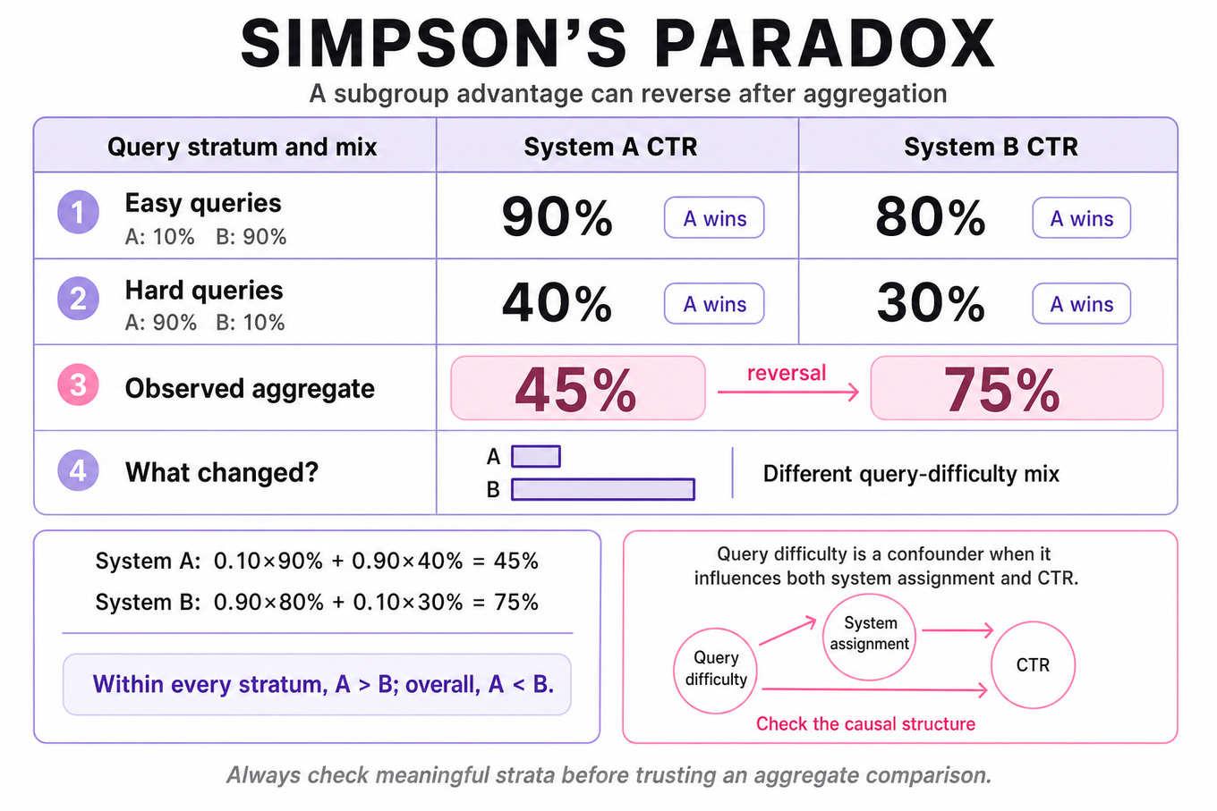
• Simpson’s paradox occurs when the direction or interpretation of an association changes after data is partitioned by a third variable. A treatment can outperform control in every subgroup yet appear worse overall because treatment and control have different subgroup proportions.

• Aggregates are weighted averages, not simple averages. For subgroup rates $r_i$ with weights $w_i$, the overall rate is $\sum_i w_i r_i$, where $\sum_i w_i=1$. A reversal is possible when the treatment groups have substantially different weights across strata.

• A confounder influences both the exposure and outcome, creating a non-causal association. For example, query difficulty may affect both ranking-system assignment and click-through rate; comparing systems without controlling for difficulty can mislead.

• Distinguish confounding from mediation and collider bias. Adjusting for a mediator can remove part of the effect you want to estimate, while conditioning on a collider—affected by both exposure and outcome—can create a spurious association.

• Start with a causal graph or explicit estimand: for example, “the average treatment effect of ranking system A versus B on qualified clicks among eligible searches.” The correct adjustment set depends on that causal question, not merely on correlated variables.

• Stratification estimates subgroup-specific effects, such as $\hat{\tau}_s=\bar{Y}_{T,s}-\bar{Y}_{C,s}$. To estimate a population effect, standardize using a common target distribution: $\hat{\tau}_{pop}=\sum_s p_s(\bar{Y}_{T,s}-\bar{Y}_{C,s})$.

• In randomized experiments, treatment is independent of pre-treatment covariates in expectation, so randomization protects against confounding. However, chance imbalance, noncompliance, differential missingness, or post-treatment conditioning can still distort practical analysis.

• For a ratio metric such as CTR = clicks / impressions, inspect numerator and denominator separately, then segment by high-impact dimensions. A change may reflect traffic mix, exposure volume, or denominator composition rather than a genuine per-impression behavioral change.

• Standardization and regression adjustment answer different operational needs. Standardization is transparent for a few important strata; regression, inverse-probability weighting, or doubly robust estimators scale better but require modeling assumptions and overlap.

• Check overlap, also called positivity: every relevant subgroup should have meaningful observations under both conditions. If one ranking system serves almost exclusively easy queries, within-stratum comparisons may be noisy or impossible.

• Statistical uncertainty matters after stratification. Small subgroups can show extreme rates by chance, so report confidence intervals or posterior intervals, account for multiple comparisons when scanning many segments, and avoid selecting only “significant” reversals.

• Not every reversal is paradoxical or erroneous. It may reflect a real population shift, a policy change, a meaningful target-population difference, or a valid difference between an overall estimand and a conditional estimand. Explain which population the metric is intended to represent.

Worked example

For “Explain and resolve Simpson’s paradox,” I would first clarify whether the interviewer wants a descriptive explanation, a causal treatment effect, or a product-metric diagnosis, and I would ask what variable defines the relevant subgroups. I would state the core pattern: an aggregate comparison can reverse because subgroup rates are weighted by different population mixes. I would organize the answer around four pillars: show subgroup tables, compute the aggregate weighted rates, identify the confounding or composition variable, and choose an estimand-appropriate resolution. For instance, if a new search system wins for both easy and hard queries but receives mostly hard-query traffic, I would not call the aggregate result a simple system failure without examining query mix. I would compare within-query-difficulty effects and then standardize both systems to the same difficulty distribution. The explicit tradeoff is that stratification improves interpretability but can increase variance or fail when some strata lack overlap; regression or hierarchical modeling may stabilize estimates while adding assumptions. I would close by saying that I would also check randomization integrity, missing outcomes, metric definitions, and confidence intervals before recommending a product decision.

A second angle

For “How do you diagnose a ratio metric change,” the same idea appears through numerator-denominator composition rather than a treatment table alone. I would decompose the ratio, compare segment-level rates and traffic weights, and test whether the overall movement is driven by a shift toward segments with systematically higher or lower baselines. The key framing is diagnostic: first establish whether instrumentation or denominator changes explain the movement, then determine whether the within-segment behavior changed. I would also distinguish an intended population change from a misleading aggregate artifact. A useful next step is to report both the observed metric and a composition-adjusted metric using a fixed reference distribution.

Common pitfalls

Pitfall: Saying “always adjust for the third variable” is analytically wrong. Adjustment is appropriate for a pre-treatment confounder, but conditioning on a collider or mediator can bias the estimand; first define the causal question and draw the likely relationships.

A tempting answer gives only a toy reversal table and declares the paradox “resolved” by averaging subgroup percentages. That ignores unequal subgroup sizes: show the weights, compute aggregate rates, and explain whether the desired quantity is the observed population effect or a standardized comparison.

Some candidates attribute every reversal to bad data or randomization failure. A stronger answer acknowledges genuine population shifts, overlap limitations, uncertainty, and multiple possible estimands, then proposes concrete checks such as segment-level confidence intervals and a pre-specified reference distribution.

Connections

An interviewer may pivot to causal diagrams, randomized experiments, inverse-probability weighting, or ratio-metric variance. Related topics include heterogeneous treatment effects, multiple-hypothesis testing, missing-data bias, and transportability from an experiment population to the product population.

Further reading

• Causality — Judea Pearl — Formal treatment of confounding, adjustment, causal graphs, and Simpson’s paradox.

• Causal Inference: What If — Hernán and Robins — Free, rigorous reference for standardization, inverse-probability weighting, and causal estimands.

• The Book of Why — Judea Pearl and Dana Mackenzie — Accessible intuition for causal reasoning and why association alone is insufficient.