Supervised ML Fundamentals, Evaluation And Feature Engineering

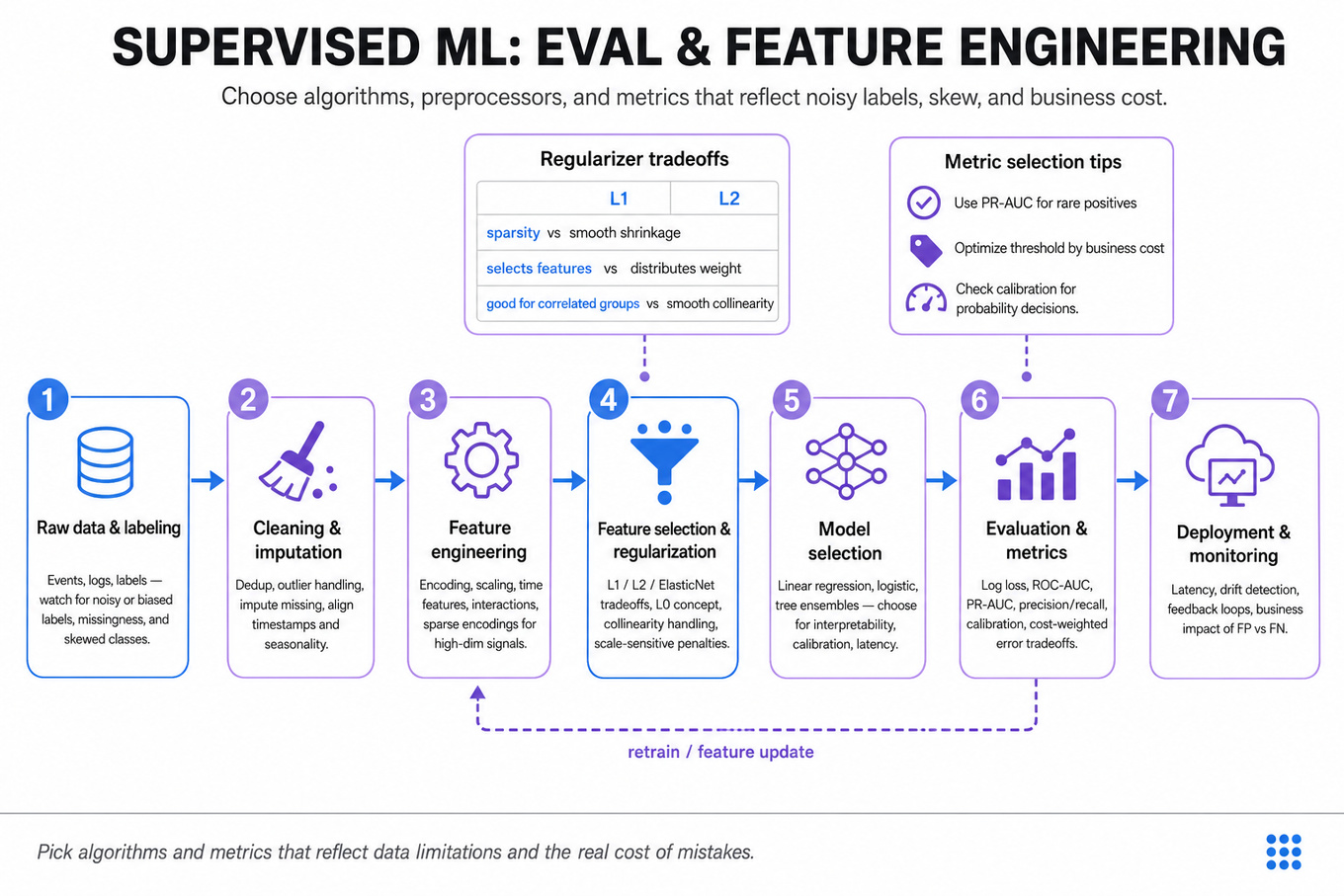
What's being tested

Interviewers are probing whether you can choose, evaluate, and explain supervised learning methods under realistic business constraints: noisy labels, skewed classes, sparse features, correlated predictors, seasonality, and metric tradeoffs. For an Amazon Data Scientist, this matters because many use cases—fraud detection, abuse prevention, conversion modeling, inventory forecasting, search relevance, and customer targeting—require defensible model choices, not just high offline scores. You are expected to reason from the data-generating process, select appropriate algorithms and metrics, identify preprocessing needs, and communicate tradeoffs clearly to product and science partners. The strongest answers connect modeling decisions to customer or business impact, such as false-positive cost, missed-demand cost, latency of decisions, or interpretability needs.

Core knowledge

• Linear regression estimates coefficients by minimizing squared error: $\min_\beta \sum_i (y_i - x_i^\top\beta)^2.$ Its classic assumptions include linearity, independent errors, homoscedasticity, no perfect multicollinearity, and exogeneity $E[\epsilon \mid X]=0$. Violations do not always make predictions useless, but they affect inference, confidence intervals, and coefficient interpretation.

• Logistic regression models class probability as $P(y=1\mid x)=\sigma(x^\top\beta)$ and minimizes log loss, not squared error. It is often a strong baseline for tabular classification, especially when interpretability, calibration, and sparse high-dimensional features matter.

• Regularization controls variance and overfitting by penalizing model complexity. L2 adds $\lambda\|\beta\|_2^2$ and shrinks correlated coefficients smoothly; L1 adds $\lambda\|\beta\|_1$ and can produce sparse feature selection; Elastic Net combines both and is useful with correlated feature groups.

• L0 regularization counts nonzero coefficients, $\|\beta\|_0$, and directly targets feature subset selection, but exact optimization is generally combinatorial. L∞ regularization constrains the maximum absolute coefficient and is less common in applied DS interviews, but tests whether you understand norm geometry and constraint effects.

• Feature scaling is essential for distance-based models, gradient-based linear models, and regularized regression because coefficients are penalized relative to feature scale. Tree models such as Random Forests, Gradient Boosted Trees, `XGBoost`, and `LightGBM` are mostly invariant to monotonic scaling, though transformations can still help with outliers or distribution shape.

• Random Forests reduce variance by bagging many decorrelated trees trained on bootstrap samples and random feature subsets. They are robust, parallelizable, and less sensitive to hyperparameters, but may underperform boosted trees on structured tabular prediction and can struggle with extrapolation beyond observed feature ranges.

• Gradient Boosting sequentially fits trees to residuals or gradients, reducing bias and often winning on tabular data. Key controls are learning rate, number of trees, max depth, subsampling, column sampling, and early stopping. It can overfit label noise if trees are deep or boosting rounds are excessive.

• Class imbalance should be handled through metrics, sampling, thresholds, and cost framing. Accuracy is misleading when positives are rare; prefer precision, recall, F1, PR-AUC, lift, recall at fixed precision, or expected cost. For a 0.1% positive class, ROC-AUC can look strong while precision is unusable.

• Threshold selection is a business decision layered on top of predicted probabilities. A fraud model might optimize expected value: $EV(t)=TP(t)\cdot B - FP(t)\cdot C - FN(t)\cdot L,$ where $t$ is the decision threshold. Always separate model ranking quality from action policy.

• Calibration matters when probabilities feed downstream decisions, capacity planning, or expected-value calculations. Logistic regression is often reasonably calibrated; boosted trees may need Platt scaling or isotonic regression. Evaluate with calibration curves, Brier score, and observed-vs-predicted rates by score bucket.

• Time-series forecasting requires respecting temporal order. Use train/validation splits such as rolling-origin evaluation, not random cross-validation. Baselines should include seasonal naive, moving average, and simple exponential smoothing before complex models like `ARIMA`, `Prophet`, `XGBoost`, or sequence models.

• Feature engineering should encode signal without leakage. For tabular Amazon-style data, common features include lagged demand, rolling means, customer tenure, frequency counts, recency, price bands, categorical target encodings, missingness indicators, and log-transformed monetary values. Compute features using only information available at prediction time.

Tip: In interviews, first state the decision context: “Am I optimizing probability accuracy, ranking quality, forecast accuracy, or a business action threshold?” This prevents generic model comparisons.

Worked example

For Compare Random Forests vs Gradient Boosting rigorously, a strong candidate would start by clarifying the prediction target, data size, feature types, class balance, label noise, interpretability needs, and whether the model is used for ranking, probability estimation, or hard classification. They might say: “I would compare these as two tree-ensemble families: Random Forests primarily reduce variance through bagging, while Gradient Boosted Trees reduce bias through sequential additive learning.” The answer should be organized around four pillars: predictive performance, robustness to noisy or missing data, tuning complexity, and evaluation metrics aligned with the business cost.

For performance, the candidate would explain that boosted trees like `XGBoost` or `LightGBM` often outperform Random Forests on structured tabular data because they iteratively correct errors, but they require careful regularization, learning-rate tuning, and early stopping. For robustness, Random Forests are a safer first pass when labels are noisy or the team needs a stable benchmark with fewer hyperparameters. For feature handling, both can model nonlinearities and interactions, but high-cardinality categoricals may require target encoding, frequency encoding, hashing, or native categorical handling depending on the implementation.

A key tradeoff to flag explicitly is that Gradient Boosting may deliver better PR-AUC or lift in the top score deciles, while Random Forests may be easier to tune and less brittle under distribution shifts. The candidate should also discuss class imbalance: use class weights, balanced sampling, calibrated probabilities, and threshold optimization rather than relying on raw accuracy. A strong close would be: “If I had more time, I’d compare both against a regularized logistic regression baseline, evaluate calibration and segment-level errors, and validate that gains persist on a temporally held-out set.”

A second angle

For Choose Models for Imbalanced Data and Time-Series Forecasting, the same fundamentals apply, but the framing splits into two separate data-generating processes. For the imbalanced classification piece, the central issue is not “which model is most accurate,” but which model ranks rare positives well and supports a defensible action threshold under asymmetric costs. For the forecasting piece, the key constraint is temporal dependence: random splits leak future information and overstate performance. A good answer would compare simple seasonal baselines, `ARIMA`-style models, tree models with lag features, and possibly hierarchical forecasting if predictions aggregate across products, regions, or fulfillment nodes. The transferable skill is matching evaluation design to the operational decision: PR-AUC or recall-at-precision for rare-event detection, and WAPE, sMAPE, pinball loss, or service-level cost for demand forecasts.

Common pitfalls

Pitfall: Treating accuracy as the default classification metric.

This is the most common analytical mistake for imbalanced problems. Saying “the model has 99% accuracy” is weak if the positive class rate is 0.5%; a trivial all-negative classifier gets 99.5% accuracy. A better answer names precision, recall, PR-AUC, top-k lift, calibration, and cost-weighted thresholding.

Pitfall: Reciting model definitions without tying them to data conditions.

A communication mistake is saying “Random Forests are better because they avoid overfitting” or “Gradient Boosting is better because it is more accurate.” Interviewers want conditional reasoning: data size, noise, sparsity, missingness, high-cardinality categoricals, latency constraints, and whether the goal is ranking, calibrated probability, or interpretability.

Pitfall: Ignoring leakage and validation design.

A depth mistake is proposing target encoding, rolling averages, or time-series features without specifying that they must be computed using only past data. For Amazon-style problems with seasonality, promotions, and customer behavior shifts, a random split can make a mediocre model look excellent. Prefer temporal holdouts, grouped splits when entities repeat, and segment-level error checks.

Connections

Interviewers may pivot from here into experiment design, especially how to validate that an offline model improvement translates into an online metric such as conversion, defect rate, or customer contacts. They may also ask about causal inference, ranking metrics like NDCG or MAP, or forecast evaluation under asymmetric costs and stockout penalties.

Further reading

• The Elements of Statistical Learning — rigorous treatment of regularization, tree ensembles, bias-variance tradeoff, and model assessment.

• An Introduction to Statistical Learning — accessible coverage of linear models, classification, resampling, feature selection, and tree-based methods.

• XGBoost: A Scalable Tree Boosting System — foundational paper explaining why regularized gradient-boosted trees became a dominant approach for tabular ML.