BCG X Data Scientist Interview: Technical Coding and Analytics Cases
Quick Overview
Prepare for BCG X data science coding and analytics cases with Australia-specific official process evidence and a clearly scoped Hong Kong candidate report. Work through an original retail stocking dataset, tested Python cost optimization, chronological evaluation and a counterexample showing why prediction accuracy and business value can disagree.
A BCG X Data Scientist interview can move from a business question to code and then back to a recommendation. Practising those pieces separately can leave you with a correct metric and no clear recommendation.
Our preparation thesis: practise an analysis you can defend from end to end. Define the decision, state what the data can support, implement a small calculation, and explain the limits of the resulting recommendation. The retail example below is original PracHub practice, not a reported BCG X question.
Use PracHub's Data Scientist questions to rehearse the technical follow-ups after completing the case.
Separate your recruiting track from general BCG advice
Official facts, Australia-specific: BCG X's associate recruitment page describes an online coding assessment, shortlisting, first-round technical interviews with cases and live coding, and additional case-based and technical interviews in the final round. Although the URL sits under an Australia-and-New-Zealand path, the current page is titled for Australia and names Australian offices and work eligibility. Do not apply that sequence to every country or experienced-hire role. BCG X's associate recruitment page.
Candidate report: a Hong Kong Data Scientist account, reported for July 2026 and published on PracHub in September, describes an assessment followed by repeated technical and business cases. It is one candidate's experience, curated and edited by PracHub, not an official BCG X process specification. The Hong Kong candidate account.
We did not establish two independent same-cycle accounts supporting one global sequence. Confirm your office, seniority, recruiting track, assessment platform, and permitted tools from the invitation. This article therefore focuses on technical-case preparation rather than promising a particular number of rounds or minutes.
Our inference: the overlap between coding and case work makes it useful to practise switching between implementation detail and business interpretation. Explain how the function's output supports the recommendation.
Turn the client problem into an explicit decision
Consider a fictional retailer choosing tomorrow's stock quantity for one perishable product at one store. The manager wants fewer missed sales without excessive leftovers.
Before discussing a model, clarify the decision time, delivery lead time, shelf life, existing usable stock, and allowable order quantities. “Forecast demand” is not yet a complete decision. The warehouse may only ship cases of four, and a late forecast may arrive after the order deadline.
For our small exercise, assume stock is chosen once per day, arrives before sales begin, and does not carry over. The decision variable is the total starting stock, not an additional order on top of existing inventory. Demand is fully observed, and each day is weighted equally.
Define a practice cost of one unit for each leftover item and three units for each unit of unmet demand. These are fictional penalty units, not a claim about a retailer's margin. They combine the costs we want the exercise to penalize without pretending we have estimated real lost-sales value.
The objective is now precise: choose a feasible integer stock quantity that minimizes average shortage and leftover penalties on the training sample. We will then evaluate that frozen choice on later days.
This is an intentionally simple decision baseline. It does not train a machine-learning forecasting model, and that is useful: it gives a more elaborate model a concrete policy to beat.
Check whether sales are actually demand
In real retail data, a store that sells all ten available items may have had demand for ten, fifteen, or more. A sales column alone cannot resolve that ambiguity. Investigate inventory availability, stockout timing, substitutions, returns, and data corrections before treating recorded sales as a complete demand label.
Our practice fixture assumes fully observed demand so the arithmetic can be checked directly. Do not quietly carry that assumption into a client dataset. Excluding every stockout day can also select an unrepresentative subset; it is a diagnostic baseline, not an automatic correction for missing demand.
Check the grain before joining tables. A store-product-day demand table joined to multiple promotion records can multiply rows and distort the sample weights. Verify uniqueness of the intended key, row counts before and after joins, and whether missing days mean zero demand or missing observation.
Then check feature availability at the decision cutoff. A promotion planned before ordering may be usable. A same-day total calculated after the store closes is not available for tomorrow-morning-style retrospective prediction unless your actual decision time permits it.
Scikit-learn's guidance describes leakage as using information unavailable at prediction time and recommends fitting learned preprocessing only on training data. That applies to imputation, scaling, and feature selection as well as the model itself. Scikit-learn's common pitfalls.
Code the decision baseline on a small dataset
Use four earlier days for training and three later days for evaluation. The dates here are represented by ordered day numbers; no seasonality or promotion variables are included.
| Split | Day | Observed demand |
|---|---|---|
| Train | 1 | 8 |
| Train | 2 | 12 |
| Train | 3 | 16 |
| Train | 4 | 20 |
| Evaluate | 5 | 10 |
| Evaluate | 6 | 18 |
| Evaluate | 7 | 22 |
Initially, allow any integer starting stock from zero through twenty-four. Break equal-cost ties by choosing the smaller quantity. Both the candidate set and tie policy belong in the contract.
def total_penalty(demand, stock, shortage=3, leftover=1):
    return sum(
        shortage * max(actual - stock, 0)
        + leftover * max(stock - actual, 0)
        for actual in demand
    )


def choose_stock(demand, candidates, shortage=3, leftover=1):
    demand = list(demand)
    candidates = sorted(set(candidates))
    if not demand or not candidates:
        raise ValueError("Nonempty demand and candidates required")
    if any(type(x) is not int or x < 0 for x in demand + candidates):
        raise ValueError("Use nonnegative integer units")
    if shortage <= 0 or leftover <= 0:
        raise ValueError("Costs must be positive")
    return min(
        candidates,
        key=lambda q: (total_penalty(demand, q, shortage, leftover), q)
    )


train = [8, 12, 16, 20]
future = [10, 18, 22]
chosen = choose_stock(train, range(25))
print(chosen, total_penalty(train, chosen), total_penalty(future, chosen))
The expected output is 16 24 30. The search evaluates a finite set of feasible decisions. With n days and k candidate quantities, scoring requires O(nk) work; sorting the candidates adds O(k log k) work. This is appropriate for a tiny practice case, not necessarily a production-scale optimizer.
total_penalty is a small arithmetic helper whose inputs follow the validated exercise contract. choose_stock rejects empty inputs, negative or noninteger quantities, and nonpositive costs. In this exercise, pass ordinary finite numeric cost values; the helper is not a complete parser for arbitrary external input.
At sixteen units, the training penalties are eight, four, zero, and twelve, totaling twenty-four. Quantities from sixteen through twenty also tie at that total under these particular data and costs. Our explicit smaller-quantity tie-break selects sixteen; a different operational preference could choose another tied feasible quantity.
Test the tie, not just the chosen output. Otherwise a later change in iteration order can silently alter the recommended stock even though the total penalty appears unchanged.
Evaluate the frozen policy on later observations
A simple comparison policy stocks fourteen units, the mean of the four training demands. Define both policies before examining the later sample.
| Later demand | Penalty at 14 units | Penalty at 16 units |
|---|---|---|
| 10 | 4 | 6 |
| 18 | 12 | 6 |
| 22 | 24 | 18 |
| Total | 40 | 30 |
On these three constructed days, sixteen units reduces the penalty from forty to thirty. That is a difference of ten penalty units, or 25% of the comparison total. It is a toy result, not an estimated production improvement or a statistically reliable effect.
Notice the trade-off: the selected policy does worse on the low-demand day and better on the two higher-demand days. The improvement follows from the asymmetric penalty contract, not from uniformly better predictions.
Do not examine the later demands, notice that twenty units would perform well, and retroactively present twenty as the training-selected decision. That would use the evaluation sample for selection. If you tune a policy on validation periods, retain a later untouched test period for the final comparison.
For a real forecasting case, use chronological evaluation aligned with the forecast horizon and the information available at each cutoff. Scikit-learn's TimeSeriesSplit provides ordered training and test splits, while its documentation notes assumptions such as equally spaced samples for comparable fold durations. A store panel still requires deliberate date and group handling. TimeSeriesSplit documentation.
Explain why lower prediction error may not win
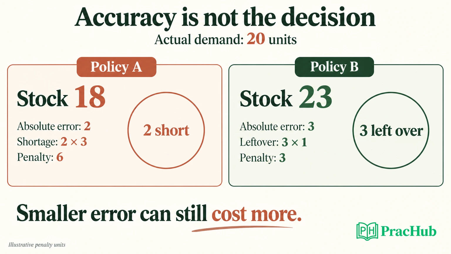
Suppose actual demand is twenty. Forecast A recommends eighteen units; forecast B recommends twenty-three. A has the smaller absolute error: two rather than three.
Under our shortage penalty of three and leftover penalty of one, however, A costs six and B costs three. The smaller prediction error produces the more expensive stocking decision.
This does not make prediction metrics useless. It means the metric must be connected to the decision. Report forecast quality alongside business penalties, availability, waste, and operational constraints. If the costs are uncertain, show how the preferred policy changes over a plausible range rather than hiding the assumption behind one score.
Change the exercise to equal shortage and leftover penalties. The optimal interval shifts, and the same smaller-quantity tie rule selects twelve. That sensitivity is a useful client discussion: the recommendation depends on what the business values, not only on which algorithm you can name.
Defend the recommendation and its limits
A concise case recommendation could be:
In this illustrative sample, a cost-aware constant-stock policy selects sixteen units and incurs thirty penalty units on the later days, compared with forty for the training-mean policy. I would treat that as a baseline worth testing, not a rollout decision. Next I would validate demand observability, confirm shortage and leftover costs, and backtest across more dates and stores before a controlled pilot.
Each sentence has a different job: identify the result, calibrate its strength, and specify the next evidence needed. Avoid changing “lower penalty in three toy observations” into “the model will reduce waste by 25%.” We measured a combined penalty, not waste alone.
If delivery cases contain four items, restrict the candidate set to feasible multiples. If capacity is fourteen, sixteen cannot be recommended even if it minimizes an unconstrained objective. If stock carries over, the decision must account for usable inventory and age; a single-day starting-stock calculation no longer describes the full problem.
For an online pilot, define the unit of assignment and possible spillovers. Customers may substitute between products or visit nearby stores, so independent product-level comparisons may miss interactions. Track service availability and waste together, keep operational overrides visible, and choose a rollback condition before launch.
If asked for a more sophisticated model, explain what additional signal would justify it: seasonality, promotions, store differences, or changing demand distributions. Start with simple baselines, compare under the same information cutoff, and separate better forecasts from a better ordering policy.
Rehearse the transitions between code and case discussion
Practise explaining the objective before writing the function, then interpret one row of the output aloud. A partner should be able to challenge the tie-break, cost ratio, capacity, or label quality without forcing you to abandon the whole analysis.
When a requirement changes, identify the affected layer. Case-pack constraints alter feasible candidates. A different shortage penalty changes the objective. Stockout-censored labels change the evidence base. Those are different problems and deserve different fixes.
Finish by stating what your code verifies and what remains an assumption. Our executable checks cover the fixture arithmetic, tie-break, feasible sets, input boundaries, and error-versus-cost counterexample. They do not establish demand identifiability, causal lift, or a production deployment's reliability.
Five questions for the next practice session
These are adjacent PracHub exercises, not a BCG X question list. Use them to challenge a specific part of the reasoning rather than memorize a company-labeled answer.
| PracHub question | What to defend |
|---|---|
| Forecast Food Stocking Needs Under Waste and Stockout Costs | Connect demand labels to asymmetric business costs. |
| Reduce Fresh-Food Waste with an End-to-End ML Approach | Determine whether forecasting or an operational change addresses the problem. |
| Choose Models for Imbalanced Data and Time-Series Forecasting | Match validation and metrics to the task. |
| Predict future time-series values | State horizon, available information, and baseline choices. |
| How would you critique this regression? | Challenge assumptions before accepting a numerical result. |
Choose another case from PracHub's Data Scientist collection, and complete the same chain: decision, data, computation, validation, recommendation.
Comments (0)