Binary Tree Right Side View: BFS Levels, Right-First DFS, and Sparse Trees
Quick Overview
Compute one visible node per depth using left-first BFS level endings or right-first DFS first visits. An original sparse six-node tree returns 8, 11, 9, 4 even though following right children stops early. Seven named cases and 2,056 ordered tree shapes match an independent root-path oracle, including repeated values and a smaller-valued right child. Width, height, parsing and iterative order are scoped separately. Five verified reported questions extend the rehearsal.
Binary Tree Right Side View asks for one existing node at each depth. A left-child-first breadth-first traversal takes the last node in every level. A right-first depth-first traversal takes the first node encountered at every new depth. Their correctness comes from the order of nodes at a depth; a visible node can be a left child.
A sparse tree exposes the distinction: the right branch can end while a deeper node in the left subtree remains visible. Use the original six-node example below to explain both algorithms, then practice related tasks in PracHub's Software Engineer coding and algorithms collection.
Evidence boundary: LeetCode's public problem defines the requested view. Python documentation supports queue and recursion details. The tree, order traces, proofs and bounded checks are original. Candidate-reported PracHub records are practice material, not evidence that an employer will use this exact exercise. Sources and links were checked on October 17, 2026.

Define visibility by depth and child order
Official problem facts: return the visible node values from top to bottom when viewing a binary tree from its right side. The public examples include an empty tree and sparse branches. The output contains values, but the decision about visibility is structural. LeetCode 199.
Here, a depth is the number of edges from the root, whose depth is zero. At a fixed depth, left-child-first level order lists existing nodes from left to right. Its final node is the one selected for the right view. Missing children contribute no value and are not queued as placeholder nodes.
The task is not to choose the numerically largest value at each level. In a root with children valued 99 on the left and negative five on the right, negative five is visible at that depth. Repeated values also remain repeated in the output when different visible nodes carry them.
It is also different from vertical traversal. Column coordinates and tie-breaking sorts answer a different ordering question. Right view needs one choice per depth; it does not group nodes into columns or sort their values.
Draw a sparse tree before choosing the traversal
Use exactly these parent-child relationships. Node three has no left child, node eleven has no right child, and node six has only a left child. The labels are identifiers for this example, not binary-search-tree constraints.
        8
       / \
      3   11
       \  /
        6 9
       /
      4
At depth two, nine lies to the right of six in level order even though nine is a left child. At depth three, four is the only existing node. The right view is therefore [8,11,9,4].
Following right pointers from the root produces only [8,11]. Choosing a right child when one exists and otherwise taking a left child would reach nine but still miss four. A single selected branch cannot reveal every depth represented elsewhere in the tree.
Ask whether a farther-right subtree has any node at the same depth. Eleven and nine cannot hide four at depth three, where their subtree has no node. This is why sparse examples reveal errors that a perfect tree with all children present may conceal.
Freeze each BFS level before appending children
A queue stores nodes waiting to be visited. To process one level, record its size before removing anything, then pop exactly that many nodes. Children appended during the loop belong to the next level and must not extend the current batch.
Append each node's left child before its right child. If the current level is ordered left to right, grouping its children's left-right pairs in that same parent order preserves the next level's order. The final popped node in the frozen batch is consequently the visible one.
def right_view_bfs(root):
    if root is None:
        return []
    queue = deque([root])
    result = []
    while queue:
        level_size = len(queue)
        for i in range(level_size):
            node = queue.popleft()
            if i == level_size - 1:
                result.append(node.val)
            if node.left is not None:
                queue.append(node.left)
            if node.right is not None:
                queue.append(node.right)
    return result
Import deque from collections before using the function. Python documents approximately constant-time appends and pops at its ends; removing index zero from a list instead requires moving the remaining items. The queue choice supports the intended linear traversal cost. Python deque documentation.
The implementation assumes a proper finite binary tree with val, left and right fields. It does not validate arbitrary object graphs for cycles or shared children. That validation is a separate input contract, not a reason to deduplicate nodes by their values.
Make the BFS ordering argument visible
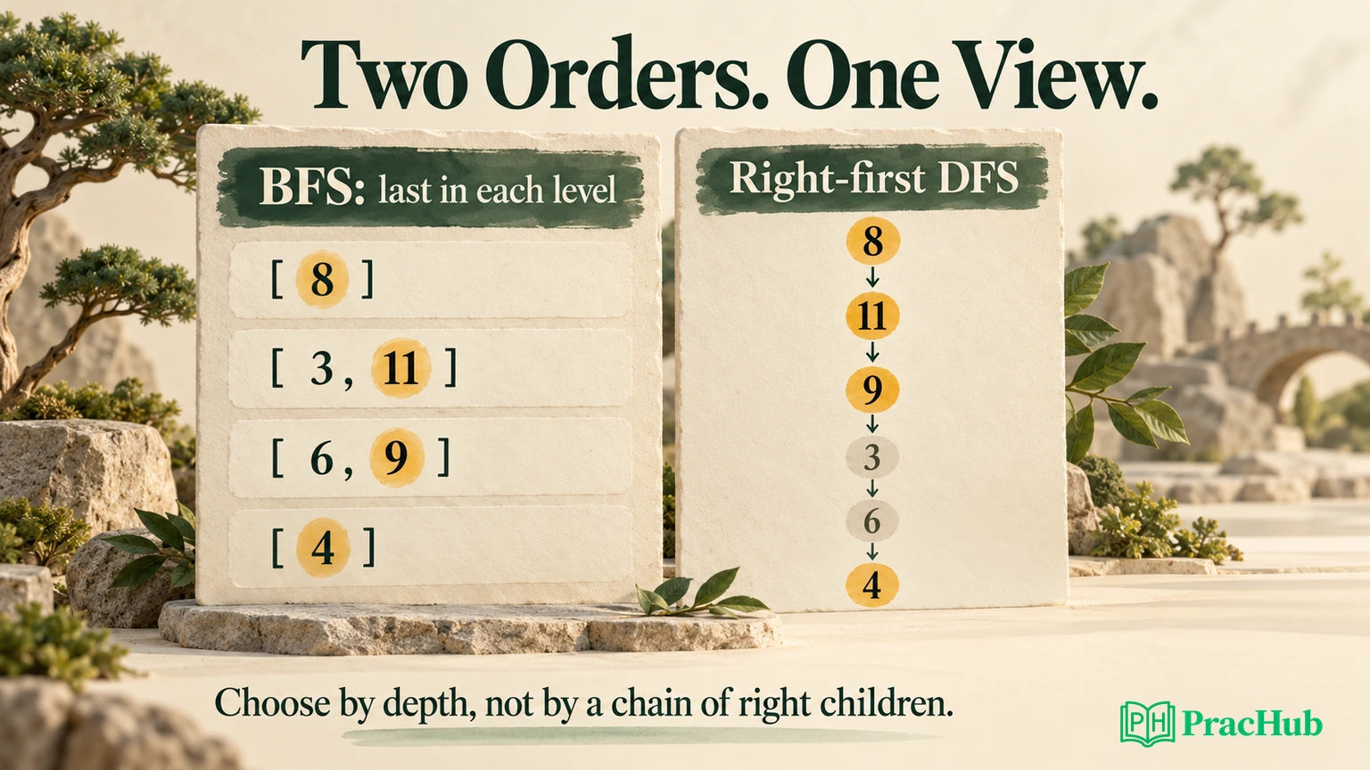
For the original tree, the successive frozen levels are [8], [3,11], [6,9] and [4]. Taking the last entry from each gives the desired view. Recording those four batches makes both the level boundary and within-level order reviewable.
If you append right children before left children, the level order reverses and the visible node becomes the first entry rather than the last. Either convention can work when the selection rule matches it. Combining right-first enqueueing with last-entry selection instead computes the opposite side.
Draining the live queue while appending children can silently combine several depths into one batch, even when every node is visited. It may consume the entire tree as one batch and return only its last visited value. Freeze level_size once at the beginning of every outer iteration.
The proof has two steps: the queue batch contains exactly the nodes at the current depth, and those nodes are ordered left to right. “BFS visits by levels” establishes only the first. The child enqueue order establishes the second and explains why the last entry is the correct one.
Let right-first DFS claim a depth once
Depth-first traversal uses a different selection rule. Visit the right subtree before the left subtree. The first node encountered at a depth is then the rightmost existing node at that depth. Record it once; later nodes at the same depth cannot replace it.
def right_view_dfs(root):
    result = []
    def visit(node, depth):
        if node is None:
            return
        if depth == len(result):
            result.append(node.val)
        visit(node.right, depth + 1)
        visit(node.left, depth + 1)
    visit(root, 0)
    return result
The length check works because a traversal cannot reach a node at a new depth without first visiting its ancestors. When depth == len(result), every shallower depth has already been represented and this depth has not. There is no need to search the result for a value.
For the sparse example, right-first preorder is 8,11,9,3,6,4. Three and six arrive at depths already represented by eleven and nine. Four reaches a previously unseen depth and is appended even though it belongs to the root's left subtree.
At a fixed depth, compare equal-length root paths at their first differing left/right choice. A path taking the right branch there belongs to the farther-right subtree. Right-first DFS explores that whole subtree first, so it encounters the winning path for each represented depth before competing paths on its left.
Preserve the order when replacing recursion with a stack
An explicit stack is last-in, first-out. To visit the right child first, push the left child first and then the right child, carrying each node's depth. Pushing the right child first reverses the intended pop order.
Keep the same “first arrival at a depth” rule. The replacement is a scheduling change, not a new definition of visibility. If you instead overwrite the answer at every encounter, left-subtree nodes visited later can replace the rightmost ones.
An alternative algorithm can traverse left first and overwrite each depth as it goes, but that also requires a separate, consistent order argument. Avoid mixing the first-visit rule from one version with the traversal order from another. State the chosen pair before debugging the implementation.
The saved fixture executes the BFS and recursive DFS versions shown above. The explicit-stack discussion is a derived follow-up, not an additional tested implementation. Python's recursion-limit documentation is relevant when the input depth can exceed the safe recursive range. Raising that limit is not the same as removing the call-stack requirement. Python recursion limits.
Compare width, height and output space
Both traversals visit every node once, giving linear time in the number of nodes. Let w be the maximum number of nodes at a level and h the number of nonempty levels. BFS needs order-w queue space; the queue can contain parts of two adjacent levels, which does not change that asymptotic bound.
Recursive DFS needs order-h call-stack space. A balanced tree can be wide but shallow, while a chain is narrow but deep. Neither method has constant auxiliary space for all tree shapes.
The returned view itself contains one value per nonempty level and uses order-h output space. State whether that output is included when comparing memory. Excluding it consistently makes the queue-versus-recursion trade-off easier to assess.
A serialized input adds parsing work and a representation contract. A compact level-order list with null markers is not automatically the same as a complete-array representation using arithmetic child indices. The examples here use explicit node links; the serialization article covers representation and validation separately.
Change the selected side without reversing depths
A request for the left view changes which node wins within each level. Left-child-first BFS should then take the first node in each frozen batch; left-first DFS should record the first arrival at each depth. The top-to-bottom order of depths remains unchanged.
For the original sparse tree, the manually derived left view is [8,3,6,4]. Reversing the right-view array gives [4,9,11,8], which reverses depth order rather than selecting the left side. This small comparison exposes a different misunderstanding from following right pointers.
If a prompt combines both sides or asks for one side in bottom-up order, state those two decisions separately. Choose the visible node at each depth first, then apply the requested depth ordering. The saved fixture executes right-view algorithms; this side-change discussion is a derived follow-up, not an additional implementation already tested.
Validate structural choices with an independent oracle
The saved local output records seven named cases and all 2,056 ordered tree shapes of zero through eight nodes passing the independent path oracle. Each shape received node labels, and both traversals were compared with an oracle that collects root-to-node left/right paths and selects the lexicographically greatest path at every depth.
That oracle uses positions rather than the BFS last-entry or DFS first-entry implementation rule. Additional cases check empty and one-node trees, chains, the sparse example, repeated values and a right child whose value is smaller than its left sibling. The last case prevents numerical maximum from masquerading as visibility.
These are bounded implementation checks, not a benchmark or proof that recursion is safe at arbitrary depth. The ordering arguments supply correctness beyond the enumerated shapes. The fixture also records the failing right-child chain separately so the original counterexample is easy to reproduce.
Practice related traversal contracts
The following PracHub records are candidate-reported tasks about right views and related traversal decisions. Some combine multiple exercises or request both sides. They are not a promise that your interviewer will use the same tree or output convention.
| PracHub question | Reported company / role | Rehearsal focus |
|---|---|---|
| Find right-side view of binary tree | Google / Software Engineer | Explain why the final left-first BFS node at each depth is visible |
| Return right and left side views of a tree | Meta / Software Engineer | Change traversal order and selection together when switching sides |
| Compute tree right view and target-sum subarrays | Meta / Software Engineer | Separate depth visibility from a subarray-sum contract |
| Produce asymmetric side views of a binary tree | Meta / Software Engineer | Clarify top-down versus bottom-up output and side selection |
| Implement right side view and local minimum search | Meta / Software Engineer | Explain the view contract independently of a second search task |
Draw the sparse tree and explain why four remains visible after the right subtree ends. Then use the verified Software Engineer coding and algorithms questions, tracing the four frozen BFS batches and the six DFS visits before explaining why a smaller-valued right child still wins.
Comments (0)