CUPED Interview Questions: Covariate Choice, Variance Reduction, and a Worked Python Example
Quick Overview
Explain what CUPED adjusts, choose treatment-independent covariates, and verify a complete fixed-coefficient Python example without promising a power gain.
CUPED interview questions test whether you can improve an experiment's precision without losing track of what makes the comparison valid. A good answer identifies a treatment-independent covariate, states how the adjustment coefficient is obtained, and explains the uncertainty calculation. “It removes noise” is only the beginning.
Use PracHub's latency experiment question to practice choosing a method after identifying the metric and randomization unit. The original Python example below makes every input visible and compares two estimators on the same users.
Evidence boundary: The method discussion draws on primary research and official documentation. All calibration observations, experiment outcomes, calculations, and preparation scenarios here are original synthetic examples. No employer assessment or universal variance-reduction percentage is implied.
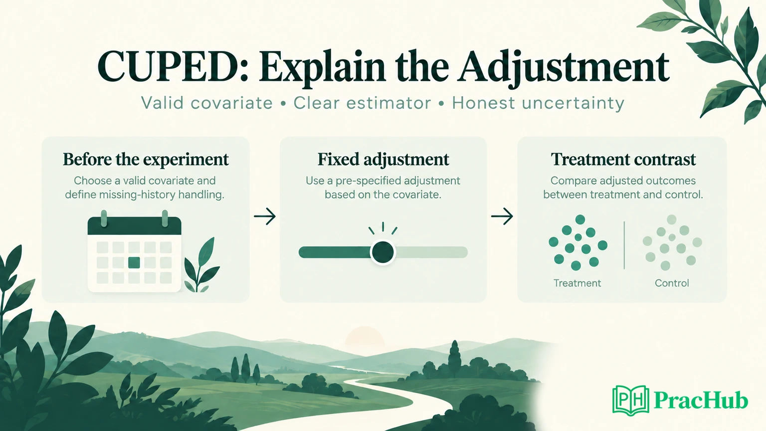
What changes when you apply CUPED?
Research context: Microsoft's experimentation team describes variance reduction as improving the treatment-effect estimator's precision. It does not mean that users themselves become less variable, nor that the experiment's assignment or telemetry problems disappear. Different metrics and product surfaces can see very different benefits. Microsoft variance-reduction overview
For a simple single-covariate adjustment, write:
adjusted outcome = Y - theta * (X - common center)
adjusted effect = mean(adjusted T) - mean(adjusted C)
Y is the experiment-period outcome, X is an eligible covariate, and theta controls how much baseline variation is removed. Because both arms use the same center and coefficient, the center cancels from the difference.
The treatment-effect target remains the difference in average outcomes under treatment and control. The adjusted estimator can differ from the raw difference in a particular random assignment because it corrects for observed chance imbalance in X.
That correction is not a license to repair nonrandom selection by adding a correlated variable. If assignment, exposure, or inclusion is biased, explain and investigate that problem directly. A narrower interval around an invalid comparison does not make it trustworthy.
Which covariate would you choose?
The original CUPED paper develops a control-variate approach using pre-experiment information and discusses covariate choice and incomplete history. In the simple linear case, the variance-minimizing coefficient is Cov(X, Y) / Var(X) for the relevant distribution. Deng and colleagues, WSDM 2013
Before estimating that relationship, inspect whether treatment could affect the covariate or its availability. A high correlation is useful for precision only after the variable passes the validity check.
| Candidate covariate | Decision and reason |
|---|---|
| Same user's activity during a fixed week before assignment | Plausible: temporally prior, with stable identity and measurement to verify. |
| Clicks on the new feature during the experiment | Reject for ordinary total-effect adjustment: treatment can change this behavior. |
| Missing history for a newly registered user | Needs an explicit policy; missing is not automatically zero activity. |
A negative correlation is not disqualifying: the coefficient can be negative. A constant covariate cannot support the covariance-over-variance calculation because its variance is zero. A weakly predictive covariate may add little practical value even when valid.
Also distinguish a pre-experiment timestamp from genuinely prior information. A feature computed later from a table that was overwritten by treatment-period behavior can leak future information despite a historical-looking column name. Check how the feature is reconstructed, not just what it is called.
Fix the coefficient before this example's experiment
Different CUPED implementations estimate coefficients differently. This original exercise deliberately uses eight independent historical calibration observations and freezes the resulting coefficient before the trial. That keeps the worked standard-error calculation separate from estimating a regression on the same small experiment.
The historical X values are [1, 2, 3, 4, 1, 2, 3, 4]; historical outcomes are [13, 15, 17, 19, 11, 13, 15, 17]. Their sample covariance divided by sample variance yields theta = 2.
These are synthetic measurements on a different calibration set, not historical rows belonging to the twelve trial users. Each trial user still has their own pre-assignment X. The distinction is between learning the coefficient elsewhere and obtaining each participant's baseline information.
A coefficient learned elsewhere is not guaranteed to be optimal for the trial population. Changes in measurement or behavior can make it less predictive. Holding it fixed makes the estimator easier to inspect; it does not remove the need to validate whether the relationship transfers.
Inspect all twelve randomized users
The example assigns exactly six of twelve users to treatment using a seeded shuffle. Each user's synthetic outcome is constructed from baseline activity, an added treatment effect of three units, and a small residual. The known construction lets us check the method without pretending the true effect is known in a real experiment.
T=1 means treatment. The common center is the full sample's mean baseline, 3.5. The following ledger shows every adjusted value:
| User | T | X | Y | Adjusted Y |
|---|---|---|---|---|
| 1 | 1 | 1 | 14 | 19 |
| 2 | 0 | 1 | 13 | 18 |
| 3 | 1 | 2 | 16 | 19 |
| 4 | 1 | 2 | 18 | 21 |
| 5 | 0 | 3 | 15 | 16 |
| 6 | 1 | 3 | 20 | 21 |
| 7 | 0 | 4 | 17 | 16 |
| 8 | 0 | 4 | 19 | 18 |
| 9 | 0 | 5 | 19 | 16 |
| 10 | 0 | 5 | 21 | 18 |
| 11 | 1 | 6 | 24 | 19 |
| 12 | 1 | 6 | 26 | 21 |
For user 1, 14 - 2 * (1 - 3.5) = 19. For user 12, 26 - 2 * (6 - 3.5) = 21. These are adjusted analysis values, not edited activity logs or claims that the users performed different actions.
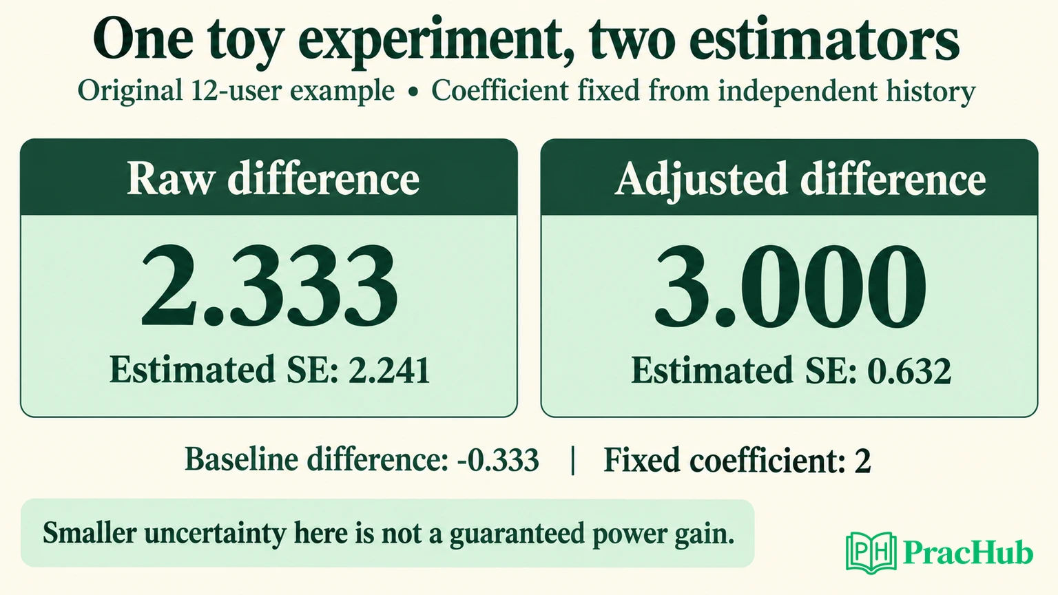
The treatment group's mean baseline is one-third of a unit below control's. The raw outcome difference is approximately 2.333. Subtracting 2 * (-0.333...) gives an adjusted difference of 3.000.
Matching the known effect exactly in this draw is a feature of this constructed example, not a general promise. In another random allocation, residual imbalance can still move the adjusted estimate away from three.
Run the calculation in Python
This complete calculation uses Python's standard library and requires no external statistical package. Implementation reference: statistics.variance and statistics.covariance compute sample quantities used below. Python statistics documentation
from statistics import mean, variance, covariance
from math import sqrt
from random import Random

# Independent, hypothetical historical calibration observations.
hx = [1, 2, 3, 4, 1, 2, 3, 4]
hy = [13, 15, 17, 19, 11, 13, 15, 17]
theta = covariance(hx, hy) / variance(hx)
assert theta == 2.0

# Complete randomization: six treated users out of twelve.
x = [1, 1, 2, 2, 3, 3, 4, 4, 5, 5, 6, 6]
treatment = [1] * 6 + [0] * 6
Random(2026).shuffle(treatment)
noise = [-1, 1] * 6
y = [10 + 2*a + 3*t + e
     for a, t, e in zip(x, treatment, noise)]
adjusted = [b - theta * (a - mean(x))
            for a, b in zip(x, y)]

def estimate(values):
    treated = [v for v, t in zip(values, treatment) if t == 1]
    control = [v for v, t in zip(values, treatment) if t == 0]
    effect = mean(treated) - mean(control)
    se = sqrt(variance(treated) / len(treated)
              + variance(control) / len(control))
    return {"effect": effect, "standard_error": se}

print("raw:", estimate(y))
print("adjusted:", estimate(adjusted))
Executed output, rounded for display:
| Estimator | Effect | Estimated SE |
|---|---|---|
| Raw difference | 2.333 | 2.241 |
| Fixed-coefficient adjustment | 3.000 | 0.632 |
The code was run and the treatment contrast was checked against the algebraic identity using the baseline difference. The full twelve-row output agrees with the ledger above.
The standard-error calculation is the square root of the sum of each arm's sample variance divided by its sample size. Apply it to the adjusted values for the adjusted contrast. Reusing the raw-outcome standard error would fail to describe the estimator you are actually reporting.
Here the coefficient is fixed independently, and the randomization unit is the individual user. For complete randomization, this is the usual two-arm Neyman variance estimate, conservative in general when individual treatment effects vary. It is an estimated uncertainty quantity, not the exact sampling standard deviation known from a single observed dataset.
Check the estimator across all possible assignments
Because the synthetic population is tiny, we can do an additional check that is impossible at production scale: enumerate all 924 ways to choose six treated users from twelve. Keep the baseline values, residuals, and constant three-unit treatment effect fixed.
Executed original verification: Across those assignments, both estimators average to 3.000. The actual randomization variance is about 4.606 for the raw estimator and 0.364 for the adjusted estimator. This verifies the expected contrast and variance reduction for this specific constructed population.
Those repeated-assignment variances are different quantities from the estimated standard errors in the single observed draw. Do not compare a variance directly with a standard error, and do not present this deliberately predictive toy population as evidence for a production traffic multiplier.
What if theta is fitted on the experiment itself?
Do not silently reuse this example's fixed-coefficient argument for a different estimator. Fitting coefficients on experiment data introduces estimation choices, including whether slopes are pooled, arm-specific, or interacted with treatment.
Microsoft's overview discusses regression-adjustment variants and their relationship to ANCOVA-style estimators. Use the inference procedure appropriate to the fitted specification and experiment design rather than treating every residualized mean comparison as interchangeable. Regression-adjustment context
In an interview, a useful answer states exactly which implementation you are discussing. For a production analysis, use a validated regression or experimentation implementation with the relevant robust or cluster-aware uncertainty calculation. Do not tune the coefficient repeatedly until the result becomes significant.
Our tiny example reports no normal-approximation confidence interval or launch decision. Six observations per arm are useful for auditing arithmetic, not for asserting that large-sample inference has automatically become reliable.
Handle missing history without changing the population accidentally
Suppose a new user has no pre-experiment activity record. Excluding that person may change the target population from all eligible users to established users. That can be a legitimate analysis if specified deliberately, but it is not the original all-user question.
One possible prespecified approach retains everyone, imputes a fixed baseline value, and includes a missing-history indicator in a suitable adjustment model. Another reports separate established-user and new-user strata with an explicitly defined combined estimand. Both require a valid missingness definition and a matching inference method.
These are editorial preparation options, not features implemented by our one-covariate script. Zero can mean observed inactivity, while missing can mean unavailable history. Treating them as equivalent without explanation may erase information about coverage.
If treatment affects whether a user joins the analysis or whether history can be linked, investigate that selection process first. “The column was measured before treatment” does not by itself guarantee that the analyzed sample was selected independently of treatment.
Explain the failure case before promising a gain
A dramatic but invalid shortcut is to use the experiment outcome itself as the covariate and subtract it with coefficient one. Every adjusted value becomes a constant, so the observed difference and estimated variability can vanish. That is not improved measurement of the total treatment effect; you subtracted the outcome you wanted to measure.
A treatment-affected engagement variable can create a subtler version of the same problem. If it sits on the pathway through which treatment changes the outcome, adjustment can remove part of the effect or induce other bias. Strong prediction does not override causal structure.
Finally, preserve the experimental unit. If teams are randomized, treating every event as an independent observation overstates information. CUPED does not fix that denominator or dependence error. Start from the assignment, outcome, and valid covariate, then choose the estimator and uncertainty calculation together.
Five questions for practicing the explanation
| PracHub question | Practice focus |
|---|---|
| Design tests to measure latency impact | Choose variance reduction only after defining the unit and outcome. |
| Estimate Experiment Duration with Power Analysis | Separate an assumed precision gain from an evidence-based power calculation. |
| Can bootstrap help reduce variance | Distinguish estimating uncertainty from changing the effect estimator. |
| Recommend a Decision After a Nonsignificant Experiment | Avoid treating a noisy result as proof of no effect. |
| Defend an Experiment Decision and Its Incremental Impact | Connect causal evidence, uncertainty, and a decision. |
These are related practice records, not a verified employer question sequence. Try the latency experiment exercise and name one valid covariate, one invalid alternative, and the uncertainty calculation you would use.
Sources and Further Reading
- Deng, Xu, Kohavi, and Walker: original CUPED paper — primary research from WSDM 2013.
- Microsoft Research: Deep Dive Into Variance Reduction — estimator precision and regression-adjustment context.
- Python statistics module — sample statistics used in the executable example.
Sources checked September 9, 2026. Numerical results describe only the original synthetic example.
Comments (0)