Machine Learning Monitoring Interview Questions: Drift, Data Quality, and Production Failures
Quick Overview
Work through a collector-key regression, mature-label cohort comparison, confusion matrices, and mix-shift counterexample to justify monitoring and recovery decisions.
An ML endpoint can return successful responses while sending the wrong tickets to the wrong team. In a monitoring interview, explaining that distinction matters more than listing drift detectors. Connect each signal to its observation window, a plausible failure, and an action you can justify.
Start with Measuring the Health of a Production ML System, From Data Quality to Business Impact, then work through the incident below. The examples are original practice exercises with fictional data, not candidate reports or claims about any employer’s interview process.
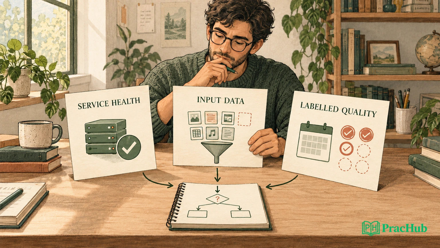
What should a production ML monitoring answer separate?
Use four layers: service health, data quality, population change, and model outcomes. Service health covers whether requests complete within the operational budget. Data quality asks whether features retain their agreed meaning. Population monitoring asks whether the observed input distribution has changed. Outcome monitoring asks whether predictions remain useful once trustworthy labels become available.
Official documentation: TensorFlow Data Validation distinguishes schema validation, training-serving skew detection, and drift detection across datasets collected at different times. These checks address different comparisons; one green check does not establish that a model is accurate.
For example, an integer feature can remain inside its permitted range while a release silently changes its meaning. Conversely, a legitimate influx of new customers can change feature distributions without breaking collection. An interview answer should explain which comparison the alert actually made, rather than treating “drift” as a complete diagnosis.
Ask for the reference population, time window, model and preprocessing versions, sample size, and label availability. Also ask what decision the prediction supports. A classifier that misses urgent support tickets needs different outcome monitoring from a model whose main cost is unnecessary specialist review.
Exercise: the endpoint works, but specialist routing deteriorates
In this fictional system, a binary classifier predicts whether a support ticket needs a specialist. The positive class means “specialist required.” Model v4 has not changed, but feature collection moved from release v12 to v13. Response status and latency remain normal. The share of requests missing prior_contacts_7d rises from 1% to 20%.
The old payload includes that key. The new collector sends contacts_last_week; the existing preprocessor reads the old key and substitutes zero when it is absent. Zero is numerically valid, so a range check alone can pass. The model now sees “no previous contacts” where history is unknown, so it can route a repeat customer as if this were their first contact.
Exercise inference: the release is a testable lead because its timing and mechanism could explain the missingness change. It is not yet proof that every wrong prediction came from the collector. A separate traffic shift or label issue could coexist.
Start with four checks:
- Break down missingness by collector version and rollout cohort, preserving request counts.
- Inspect an authorized, redacted sample at the collection boundary and after preprocessing.
- Replay the same sample through both preprocessing versions and compare feature values and missing indicators.
- Check whether the monitoring job itself changed its reference data or aggregation.
Official engineering guidance: Google’s Rules of Machine Learning discusses training-serving skew and recommends checking the relationship between serving features and training data. That supports inspecting the actual feature path; it does not establish the cause of this fictional incident.
Record the feature contract in terms a test can check: the key name, units, lookback boundary, timezone, missing-value policy, and source freshness. A seven-day contact count calculated in local calendar days may differ from a rolling 168-hour window. Correct types do not resolve that semantic disagreement. Include examples at window boundaries and distinguish a genuine zero from an unavailable history.
For the replay, hold model weights and payloads constant while changing one preprocessing implementation. If feature outputs differ, inspect where they diverge before comparing final predictions. If they agree, the collector hypothesis needs more evidence. This is more informative than rerunning a large evaluation with several components changed at once.
The proposed response is to restore the feature contract if reproduction confirms the mismatch and a supported rollback is available. Retraining immediately would risk teaching a replacement model from corrupted inputs. Preserve incident evidence before rollback, and verify that missingness recovers afterward. Model quality may take longer to confirm because labels arrive later.
How do delayed labels change the evaluation window?
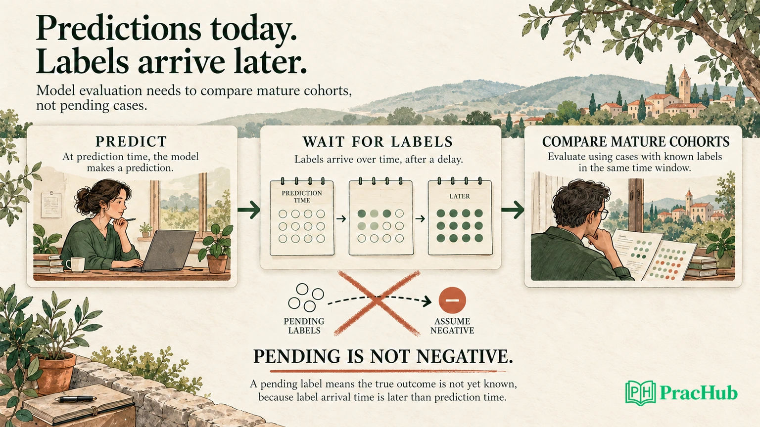
Use a prediction cohort: requests grouped by when predictions were made, not simply labels received today. This exercise assumes labels become final seven days after prediction. That is a fictional business rule, not a universal maturity period.
| Prediction cohort | Evaluation date | Final labels available | What can you conclude? |
|---|---|---|---|
| October 1: 1,000 predictions | October 8 | 1,000 | Evaluate this mature cohort. |
| October 8: 1,000 predictions | October 9 | 200 | Describe the labelled subset and coverage; full-cohort quality remains unknown. |
| October 8: 1,000 predictions | October 15 | 1,000 | Compare with the earlier mature cohort, subject to comparable definitions and populations. |
Suppose 50 of the 200 early-labelled predictions are wrong. Their observed accuracy is 75%. Comparing that directly with the earlier cohort’s full accuracy mixes label maturity with performance. Cases resolved quickly might be easier, harder, or selected by the model’s own routing decisions. The direction of bias is not known from coverage alone.
Pending labels are not negative labels. Do not fill them with zero or assume that no complaint means a correct prediction. Report coverage by prediction age, route, and relevant segment. If some outcomes never become observable, explain that selection problem rather than waiting indefinitely for a supposedly complete cohort.
Official implementation example: AWS’s model-quality monitoring documentation describes merging captured predictions with ground truth before evaluation. The page currently says Model Monitor is closed to new customers, so this is evidence for the evaluation contract, not a recommendation to adopt the service.
Keep evaluation features separate from post-outcome information. If the final specialist disposition later flows back into a historical feature table, rebuilding old features from that table can make the model appear more accurate than it was at prediction time. Preserve the feature values actually served, or reconstruct them with an explicit point-in-time rule. The monitoring query itself deserves review: a correct metric formula applied to leaked or mismatched rows still gives an unreliable answer.
Your join needs a stable prediction identifier and an explicit policy for retries or repeated predictions. Keep prediction time, model version, preprocessing version, decision threshold, label event time, label arrival time, and label revision. A corrected label should replace or version the original outcome under the evaluation policy; it should not silently create a second observation. Otherwise, apparent improvement could come from duplicate joins or a changed denominator.
Which metrics reveal the actual failure?
Once both cohorts mature, the exercise produces these counts at the same decision threshold:
| Count | October 1 cohort | October 8 cohort |
|---|---|---|
| True positives | 160 | 120 |
| False negatives | 40 | 80 |
| False positives | 80 | 80 |
| True negatives | 720 | 720 |
| Total predictions | 1,000 | 1,000 |
Official metric definitions: scikit-learn’s classification metrics documentation defines precision and recall from these counts. Applying those definitions, accuracy falls from 88% to 84%; specialist recall falls from 80% to 60%; precision falls from about 66.7% to 60%.
“Accuracy dropped four points” hides the workload consequence. Missed specialist cases doubled from 40 to 80. If specialist need is the outcome the business cares about, recall and missed-case volume make that failure visible. Precision still matters because a response that routes everything to specialists could overwhelm the team.
Do not declare a release causal from this table alone. Both cohorts contain 200 positives, but that does not establish equivalent difficulty, equal label quality, or comparable customer mix. Inspect the version-linked reproduction and segment results alongside the mature outcome evidence.
An interviewer may ask for one monitoring metric. Give a primary decision metric, then name its guardrails: for this scenario, specialist recall with review volume, precision, label coverage, and service availability. Define the operating threshold and business cost before proposing a universal alert cutoff.
Can aggregate quality fall while every segment stays unchanged?
Yes. Consider a separate fictional calculation. Segment A maintains 95% accuracy and segment B maintains 75%. A baseline containing 800 A requests and 200 B requests has 91% overall accuracy. A later cohort containing 200 A and 800 B requests has 79% overall accuracy, even though neither segment deteriorates.
Reweight both periods to a fixed 50/50 mix and each scores 85%. This does not erase the lower live accuracy: the system genuinely handles a harder mix of requests. It changes the explanation and possible response. Capacity planning, routing policy, or model coverage may be more relevant than investigating a regression inside either segment.
Distinguish input drift from concept drift. Changed input distributions alone do not prove that the relationship between inputs and outcomes changed. Where labels are available, inspect performance within meaningful slices and compare how outcomes relate to features. Where labels are unavailable, be explicit that concept drift remains a hypothesis.
Slices also have limits. Tiny groups produce unstable estimates, and searching many slices can surface chance extremes. Choose important slices before the incident where possible, retain denominators, and investigate uncertain signals before treating them as established regressions.
What makes an alert actionable rather than noisy?
Attach an owner, reference definition, freshness check, and next diagnostic step. A missingness alert should say which feature changed, in which release cohort, and how many predictions were affected. “Drift score high” leaves the responder to reconstruct the problem during an incident.
Ask how the reference was chosen. Comparing Monday morning with a quiet Sunday night can produce a predictable alert. A training baseline answers a different question from last week's corresponding production window. Save the baseline identifier so an updated reference cannot silently make an incident disappear. Rebaseline only after understanding the change and recording what the new comparison will stop detecting.
A statistical test also needs interpretation. With enough observations, a small distribution difference can be statistically detectable but operationally harmless. With few observations, a harmful change may remain uncertain. Pair statistical evidence with effect magnitude, affected prediction volume, and a diagnostic slice. Do not turn a named drift test into an automatic retraining policy.
Thresholds should reflect volume, normal variation, and the cost of delay. A rare segment may need a longer observation window; a broken required field may justify immediate intervention. Monitor missing monitoring data too. A dashboard that stopped receiving predictions must not present yesterday’s green status as today’s health.
For this exercise, a defensible response sequence is:
- Investigate and contain the reproduced collector contract failure.
- Verify restored feature values and missingness on new traffic.
- Follow mature prediction cohorts to check specialist recall and workload.
- Consider retraining only after confirming usable data and a reproducible evaluation comparison.
Keep fallback behavior explicit. Sending more tickets to human review may protect recall but consumes capacity. Disabling automation can also delay service. Explain the trade-off, who authorizes it, and how the team will know when to restore normal routing.
How should you demonstrate the reasoning in an interview?
Draw three artifacts: the feature path, the cohort ledger, and the confusion matrix. Together they show where a failure enters, which outcomes are observable, and why the response matters. Start with the decision, then describe the smallest check that could change it.
A concise answer might be: “I would first compare missingness by collector version and replay the same payload through preprocessing. Current accuracy is provisional because only 200 labels are available. If the key mismatch reproduces, I would restore the feature contract, then evaluate mature cohorts for specialist recall and review volume.”
Recalculate the confusion matrices and fixed-mix example yourself. Then write the cohort eligibility rule: the prediction is old enough under the stated policy, its label is final, and that label had arrived by evaluation time. Reject duplicate prediction IDs until the retry or version policy explains them.
Use these follow-ups to test a different weakness each time:
| PracHub practice question | What to explain |
|---|---|
| Measuring the Health of a Production ML System, From Data Quality to Business Impact | Separate operational, feature, outcome, and business signals. |
| Diagnose Strong Validation and Weak Production Performance | Test serving mismatch before blaming the algorithm. |
| Redesign a Spam Classifier for Production | Connect threshold choices to error costs and capacity. |
| Auditing a Dataset for Sampling, Measurement and Label Bias Before Relying on It | Explain which outcomes your evaluation never observes. |
| Debug a Machine Learning Pipeline | Isolate a broken boundary with reproducible evidence. |
For a focused rehearsal, answer Diagnose Strong Validation and Weak Production Performance aloud. State your first diagnostic check, the result that would change your response, and the evidence you would wait for before declaring recovery.
Comments (0)