MATLAB Interview Questions: Matrix Operations, Indexing, and Numerical Checks
Quick Overview
MATLAB interview preparation through an original sensor-data case: distinguish element-wise calibration from matrix projection, trace column-major indices, align row masks and timestamps, preserve missing values, handle complex transpose and defend numerical tolerances. Includes worked results and an original script checked in GNU Octave; MATLAB language claims link to MathWorks documentation.
MATLAB interview questions become easier to explain when you name what each axis means before choosing an operator. Separate channel-wise arithmetic from matrix multiplication, trace indexing order, and check numerical results against a stated policy. Matching dimensions alone cannot establish that an operation answers the intended question.
This article uses an original sensor-data exercise with worked outputs. MathWorks documentation supplies the MATLAB language facts. The accompanying script was executed locally in GNU Octave 11.3.0; MATLAB itself and its toolboxes were not run. These exercises are teaching material, not reported questions from a particular employer.
Start with PracHub’s matrix multiplication complexity question if you need to rehearse the mathematics. The exercise below adds the MATLAB decisions that a generic matrix algorithm leaves open.
What do the rows, columns and missing values represent?
An array contract states the dimensions, meaning of each axis, data type and treatment of exceptional values. For this exercise, rows are four consecutive time samples, columns are three sensor channels, and numeric values use ordinary double precision. NaN marks one missing observation; it is not a measured zero.
S = [1 10 100;
     2 20 NaN;
     3 30 300;
     4 40 400];
t = [0; 1; 2; 3];
gains = [2 0.1 0.01];
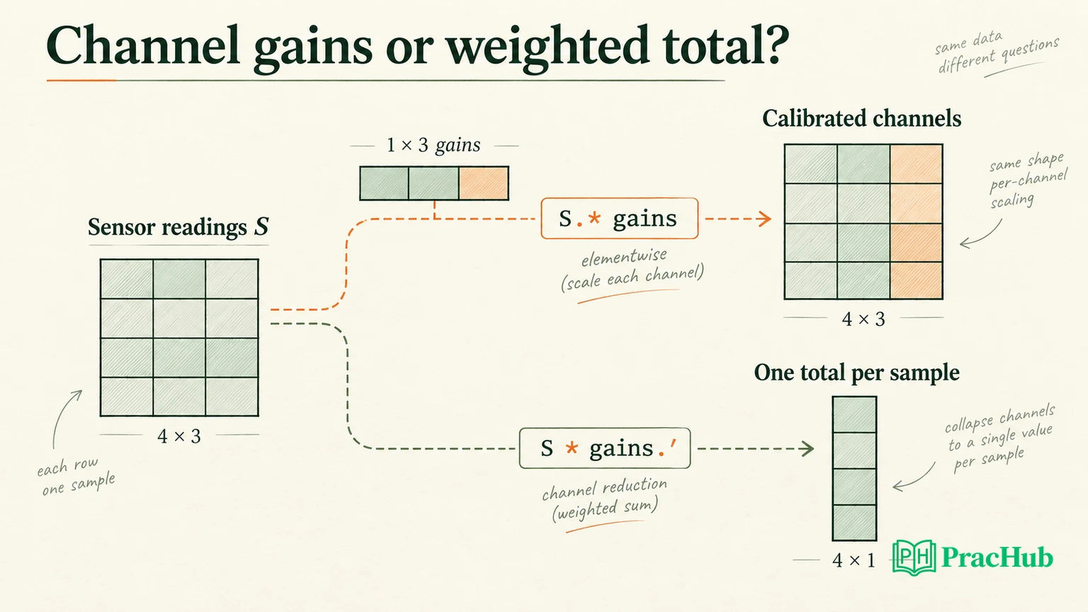
The task is to apply one calibration gain to each channel while preserving all four sample rows. A separate task asks for one weighted total per sample. Both use the same numbers, but they require different operations and output shapes.
Ask whether missing observations should remain visible, exclude a complete sample or be imputed under a defined rule. Here, calibration preserves the missing value, and a later selection excludes incomplete rows. We do not infer a real sensor’s units, calibration quality or physical accuracy from these invented values.
When do you use .* instead of *?
Official MATLAB semantics: .* multiplies corresponding elements and expands compatible sizes. A 1×3 gain row therefore applies one value to each column of our 4×3 data. This concerns compatible dimensions; it does not decide which axis the gains should belong to. MathWorks times reference
Y = S .* gains;
% Y = [2 1 1; 4 2 NaN; 6 3 3; 8 4 4]
Explain one element: Y(3,2) is 30*0.1, so it is 3. The result remains 4×3, and the second row’s missing third channel remains missing. The language cannot tell whether these gains belong to channels or samples; that meaning comes from the contract.
Official MATLAB semantics: * is matrix multiplication, with matching inner dimensions. For a weighted total across channels, multiply S by a 3×1 gain column. MathWorks mtimes reference
projection = S * gains.';
% projection = [4; NaN; 12; 16]
The first output is 1*2 + 10*0.1 + 100*0.01 = 4. It is one scalar per sample, not three calibrated readings. S*gains fails because 4×3 and 1×3 do not have matching inner dimensions. Transposing until code runs is insufficient: name the intended output before changing orientation.
How do you predict a linear index without reading row by row?
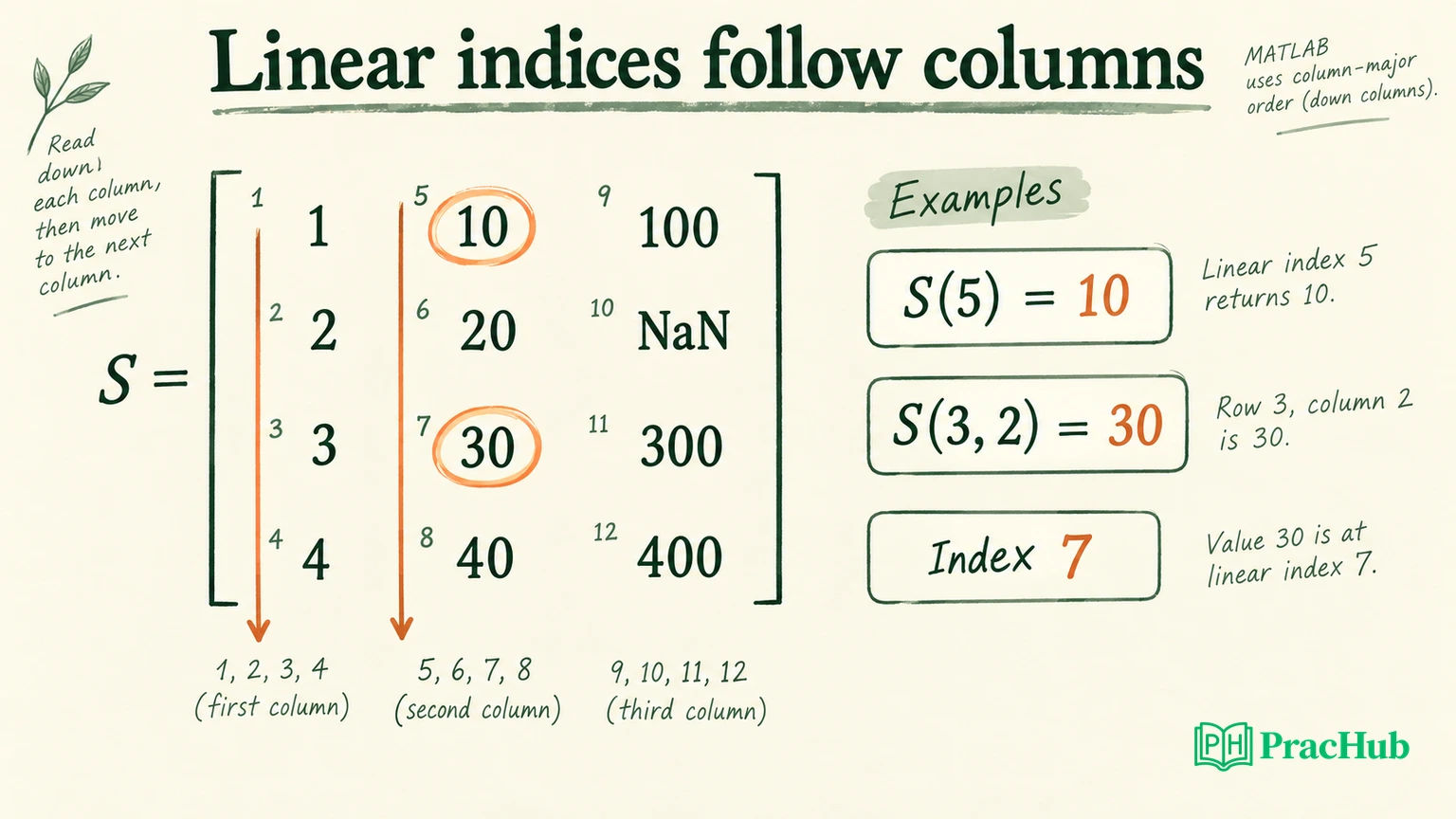
Official indexing rule: MATLAB linear indexing follows columns. For this four-row fixture, position (row, column) maps to row + (column-1)*4. S(5) therefore means the first row of the second column, which is 10; S(3,2) is 30 at linear index 7. MathWorks array indexing
S(:)
% [1;2;3;4;10;20;30;40;100;NaN;300;400]
sub2ind(size(S), 3, 2)    % 7
Read down each column; scanning the displayed rows gives the wrong linear order. Write the four elements of column one before moving to column two. This predicts both a single-index access and the order of a flattened result.
As a rehearsal variation, change the number of rows. The stride in the formula then changes too; do not memorize that the second column always starts at index five. Use size(S,1) or sub2ind when translating coordinates in code, and retain the axis meaning when you later reconstruct a matrix.
Does a logical mask preserve the sensor layout?
For our fixture, mask = S > 25 selects values 30, 40, 100, 300 and 400. Their linear positions are 7, 8, 9, 11 and 12. S(mask) extracts those values as a column vector; it does not retain a rectangular four-sample, three-channel layout. This is an application of the documented logical-indexing behavior, not another kind of calibration.
mask = S > 25;
selected = S(mask);
% selected = [30;40;100;300;400]
If the task instead asks for complete sample rows, build a row mask and use it on both the readings and their timestamps:
validRows = all(isfinite(S), 2);
completeSamples = S(validRows, :);
completeTimes = t(validRows);
% completeTimes = [0;2;3]
The shared row mask keeps samples one, three and four aligned with times zero, two and three. Removing bad values separately from each channel would destroy the relationship between channels and sample times. Filtering only S while leaving t untouched creates a different alignment error, even if both variables still look plausible when printed.
How should you handle NaN in a derived quantity?
Our original requirement is to preserve missingness during calibration. If sample energy is the sum of squared calibrated channel values, use element-wise powers and reduce across columns:
energy = sum(Y.^2, 2);
% energy = [6;NaN;54;96]
For the first sample, 2^2 + 1^2 + 1^2 = 6. The second sample remains unknown because one contributing channel is missing. Y^2 attempts a matrix power rather than squaring each reading; this nonsquare matrix is not a valid input for that operation. Array and matrix operators
Ignoring missing values would answer a different question: energy over the available channels, rather than energy over all three required channels. Replacing missing data with zero also changes the observation. Either may be appropriate under another specification, but neither should happen silently to make an assertion pass.
Test the all-missing case, an infinite observation and the case where every row is excluded before adding this policy to a larger pipeline. Decide what an empty selection should return and whether later calculations accept it. The small fixture establishes our chosen behavior; it does not validate a complete acquisition system.
Why are ' and .' different for complex data?
Official MATLAB semantics: .' is the nonconjugate transpose. It exchanges rows and columns without changing imaginary signs; ' also conjugates complex values. They agree for the real gain vector above but differ for complex sensor or signal data. MathWorks transpose reference
q = [1+2i; 3-4i];
q.'    % [1+2i  3-4i]
q'     % [1-2i  3+4i]
Explain whether you want orientation alone or a conjugate inner product. Replacing a dimension fix with the wrong transpose would conjugate the two imaginary components in this example. Include a deliberately complex test if the function’s contract permits complex data; an all-real fixture cannot expose this distinction.
What numerical comparison is defensible?
Official numerical fact: MATLAB floating-point numbers have finite precision, and some decimal values cannot be represented exactly. A printed decimal is not proof of exact equality. MathWorks floating-point explanation
Our original comparison policy combines an absolute allowance near zero with a relative allowance that scales with the expected magnitude:
actual = 0.1 + 0.2;
expected = 0.3;
tolerance = 1e-12 + 1e-10 * abs(expected);
closeEnough = abs(actual - expected) <= tolerance;
The local run produced an absolute difference of about 5.55e-17, below this policy’s 3.1e-11 allowance. Exact equality was false, while closeEnough was true. The deliberately incorrect value 0.3001 failed the same comparison.
These tolerances are exercise choices, not MATLAB defaults or universal engineering limits. Select them from the required accuracy, magnitude and data type. Check missingness, infinities and shape separately; a tolerance cannot rescue a wrong axis, and an overly generous threshold can conceal a substantial error.
How do you check a linear-system answer?
Official MATLAB behavior: A\b solves a linear system. A square system, a rectangular least-squares problem and a singular system need different interpretations; a returned result is not automatically reliable. MathWorks mldivide reference
For an independent tiny example:
A = [2 1; 1 3];
b = [1; 2];
x = A\b;                       % approximately [0.2;0.6]
residual = norm(A*x - b, inf);
assert(residual <= 1e-12);
Substitute the proposed values into both equations: 2*0.2+0.6=1 and 0.2+3*0.6=2. That gives a transparent hand check alongside the local residual. Use the solve operator to express the task directly.
A small residual alone does not guarantee a small solution error for an ill-conditioned problem, as MathWorks’ reference explains. State what your check establishes and inspect relevant warnings and conditioning before generalizing. This example verifies a small, well-behaved system; it is not a benchmark of solver performance.
What changes when the caller supplies unexpected data?
Our fixture assumes a numeric 4×3 matrix and a gain for each of three channels. Before adapting it into a reusable function, decide which dimensions are fixed and which may vary. A function accepting any sample count still needs agreement on the channel count, timestamp count and gain orientation. A row vector of three readings could mean one sample, while a column vector could mean three samples of one channel. Reshaping either automatically would hide that ambiguity.
State whether the interface accepts complex values, integer arrays and an empty batch. The examples here do not establish behavior for every input class. Converting an input to double precision may be a deliberate design choice, but it does not supply missing units or recover precision already lost upstream.
Explain the order of your checks: reject an invalid contract, perform the intended operation, then compare the output against the appropriate shape, missing-value policy and numerical allowance. If an interviewer asks for faster code, first preserve those requirements in the proposed change. A compact vectorized expression is useful when its meaning remains clear; its brevity alone supplies no evidence about runtime or memory use. Measure a representative workload before claiming a speedup.
Which checks should you explain after fixing the code?
Download the original sensor exercise and execution record. Run sensor_interview from its directory. The accompanying original sensor_interview.m passed 27 checks in GNU Octave 11.3.0. They cover dimensions and values, linear order, selected positions, timestamps, missing energy, complex transposes, tolerance acceptance and rejection, unchanged input, three expected failures and the linear-system residual. This is actual local execution in Octave; MATLAB-specific runtime behavior remains untested.
| Expression or check | Result in the original exercise | What it establishes |
|---|---|---|
S .* gains | 4×3; third-row second value 3 | One gain per channel |
S * gains.' | 4×1; first value 4 | One weighted total per sample |
S(5) / S(3,2) | 10 / 30 | Column-major index reasoning |
S(S>25) | [30;40;100;300;400] | Extraction order and shape |
t(validRows) | [0;2;3] | Shared sample selection |
S*gains, Y^2, S(13) | Each raises an error locally | Rejection of three invalid operations |
For a stronger rehearsal, explain the rejected expression before showing its correction. Then change one assumption: a different sample count, a missing channel or complex inputs. State which checks should still pass and which expected outputs must change. Avoid claiming that a successful script validates real sensor calibration or MATLAB toolbox behavior.
Practise transferable questions with explicit boundaries
These verified PracHub records extend the reasoning. They are not a dedicated MATLAB assessment bank, and some use other languages or representations. Use them to explain mathematics and checks rather than assume identical syntax.
| PracHub question | Practice focus |
|---|---|
| Analyze matrix multiplication complexity | Inner dimensions and work per output |
| Compute Prefix Matrix Products | Multiplication order and intermediate results |
| Implement a Sparse Matrix Class | Representation and value checks; not MATLAB sparse API practice |
| Compute and Explain Mean and Variance | Numerical definitions and validation |
| Explain linear algebra for graphics transforms | Orientation and the meaning of a matrix operation |
Try Compute Prefix Matrix Products by predicting an intermediate shape and one value before executing code. For the sensor exercise, use the same habit, then check indexing and numerical policy. For each answer, name the operation, predict one output and state what your check leaves untested.
Sources and Further Reading
- MathWorks: array and matrix operations
- MathWorks: element-wise multiplication and compatible sizes
- MathWorks: matrix multiplication
- MathWorks: positional, linear and logical indexing
- MathWorks: nonconjugate transpose
- MathWorks: floating-point representation and precision
- MathWorks: linear systems and mldivide limitations
Documentation checked October 11, 2026. All data and exercises are original teaching fixtures; local execution used GNU Octave, not MATLAB.
Comments (0)