Robot Inverse Kinematics Interview: Multiple Solutions, Joint Limits, and Continuity
Quick Overview
Solve robot inverse kinematics with checked two-link branches, joint limits and waypoint continuity, then explain singularity and trajectory boundaries. Primary references, original worked assets and explicit evidence boundaries support focused interview practice.
Robot inverse kinematics interview questions should end with a feasible configuration, not just an angle formula. Generate the possible branches, reject solutions that violate joint constraints, verify the remaining angles with forward kinematics, and choose continuity relative to the previous configuration. A reachable Cartesian point does not automatically imply a safe or executable trajectory.
The primary robotics references below explain analytical and numerical IK. The two-link arm is an original Python-checked exercise with explicit lengths and limits; no physical arm or production motion planner was run. Use PracHub's unicycle kinematics simulation question to rehearse model assumptions, while recognizing that a mobile robot's motion model differs from the manipulator solved here.
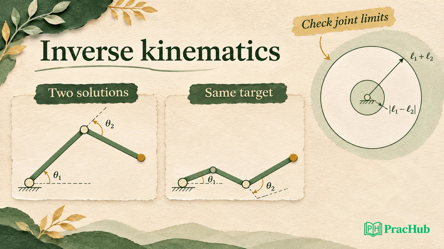
Define the task and the arm before solving it
The original arm has two revolute joints in a plane. Link lengths are L1 = 1.0 meter and L2 = 0.8 meters. The shoulder angle q1 is bounded from −90 to 90 degrees; the relative elbow angle q2 is bounded from −140 to 140 degrees. The end-effector task specifies position x/y only, not orientation.
This last distinction matters. A two-joint arm generally cannot satisfy an arbitrary planar position and an additional independent end-effector orientation simultaneously. If the interviewer adds orientation, revise the task or mechanism instead of quietly reusing the position-only answer.
Forward kinematics for this model is:
x = L1*cos(q1) + L2*cos(q1 + q2)
y = L1*sin(q1) + L2*sin(q1 + q2)
The formulas use radians in computation. Convert to degrees only for the displayed table and limit checks if your implementation chooses that convention. Mixing units can produce plausible-looking but incorrect configurations, especially when small angles appear in a test.
Official background: the Illinois Robotic Systems IK chapter develops the two-link solution and discusses constraints, singularities and numerical methods. Our lengths and bounds are supplied exercise inputs, not specifications of a particular robot.
Derive both elbow branches for one target
For the target (1.2, 0.4), use the law of cosines:
c2 = (x*x + y*y - L1*L1 - L2*L2) / (2*L1*L2)
q2 = +acos(c2) or -acos(c2)
q1 = atan2(y, x) - atan2(L2*sin(q2), L1 + L2*cos(q2))
The target's squared distance is 1.60. Subtracting 1.00 and 0.64, then dividing by 1.60 gives c2 = −0.025. The two elbow angles are approximately +91.4325 and −91.4325 degrees.
| Branch | Shoulder q1 | Elbow q2 | Within supplied limits |
|---|---|---|---|
| Positive elbow angle | −20.7820° | +91.4325° | Yes |
| Negative elbow angle | +57.6518° | −91.4325° | Yes |
Both configurations reach the same Cartesian target, but their elbows occupy different positions. “The IK answer” is therefore a set until an additional selection criterion is supplied. Choose a branch using a stated objective, rather than array order.
The local fixture substitutes each accepted solution into the forward equations and checks position error below 1e−10 meters. The residual checks numerical consistency within this model. It is not a measured positioning accuracy, and it says nothing about encoder calibration, link flex or obstacles.
If an interviewer asks why atan2 matters, explain that it preserves quadrant information and handles the geometry of the angle difference. Replacing it with a bare arctangent ratio loses information and introduces division-by-zero problems that are avoidable in this derivation.
Distinguish unreachable from joint-limit rejected
Without joint limits, a two-link position lies in an annulus: its distance from the base must be between |L1 − L2| and L1 + L2. Here that is 0.2 to 1.8 meters. This is a geometric reachability condition, not the complete constrained workspace.
The target (2.0, 0) lies outside the outer radius, so return an unreachable status before evaluating acos on an invalid value. The target (0.3, 0) is inside the annulus, but its elbow solutions exceed the supplied ±140-degree bound. Return joint-limit rejected rather than pretending the arm cannot geometrically reach it.
| Target | Unconstrained geometry | Constrained result | Useful diagnosis |
|---|---|---|---|
| (1.2, 0.4) | Two branches | Two valid solutions | Choose using a further objective |
| (0.3, 0) | Inside the annulus | No solution within the elbow limits | Constraint rejection |
| (2.0, 0) | Beyond maximum reach | No solution | Unreachable target |
| (1.8, 0) | Fully extended boundary | One distinct solution, (0°, 0°) | Singular configuration |
For floating-point arithmetic, use a small tolerance near ±1 before clamping c2 into the legal inverse-cosine range. A value of 1 plus roundoff is different from a clearly unreachable target. Do not clamp every invalid value indiscriminately; that silently moves an impossible target onto the reachable boundary.
At the fully extended point, the positive and negative elbow branches coincide. Deduplicate them within a declared tolerance. Reporting two numerically identical solutions overstates the available choice.
Choose continuity from a previous configuration
Now supply a seed configuration of (60°, −90°). The task is to follow three nearby waypoints: (1.2, 0.4), (1.18, 0.45) and (1.15, 0.5). Both branches remain within the limits, but the negative-elbow branch is much closer to the seed.
The original selection rule minimizes the squared joint-angle change among feasible candidates at each waypoint. It then uses the selected configuration as the next seed. This is a local continuity policy, not a globally optimal trajectory planner.
| Waypoint | Selected q1 | Selected q2 | Joint-space step from previous configuration |
|---|---|---|---|
| (1.2, 0.4) | 57.6518° | −91.4325° | 2.7506° |
| (1.18, 0.45) | 60.1623° | −91.6152° | 2.5171° |
| (1.15, 0.5) | 63.0963° | −92.4179° | 3.0418° |
The final column is the Euclidean norm of the two angle changes, not a maximum joint speed. Without timestamps, you cannot convert it into a velocity requirement. Label the step metric beside the values.
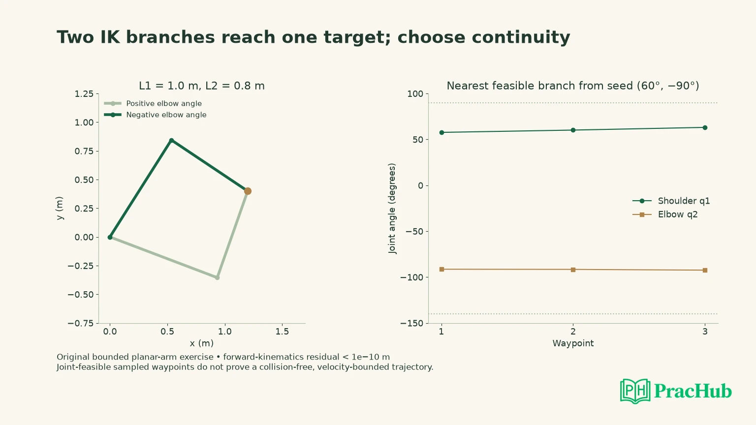
These joints are bounded, so the fixture compares the legal angle coordinates directly. For a continuously rotating joint, an angular distance may need periodic equivalence. For a bounded joint, wrapping across a forbidden range can claim a short motion that the mechanism cannot perform. Respect the actual joint type rather than applying one angle-normalization helper everywhere.
Explain where a greedy branch choice can fail
Selecting the closest feasible configuration at each waypoint works for this small trace. It can fail when the locally attractive branch approaches a limit, obstacle or singularity that a different earlier choice could avoid. A seed-sensitive numerical solver can also converge to a different branch after a small target change.
For a longer path, consider candidate configurations and transitions together. Reject transitions that violate limits or collision constraints, then choose a sequence under an explicit objective. If no valid transition remains, report that failure instead of jumping to a distant branch and calling it continuous.
The Klampt IK documentation provides official implementation context for numerical IK objectives and solver behavior. A numerical failure from one seed is not automatically proof that the target is globally infeasible. Conversely, a solver's success flag still needs interpretation against the task, residual and constraints you requested.
Ask what should happen when a waypoint has no acceptable solution: stop, replan, relax a task constraint, change the target or escalate to a higher-level policy. Silently returning the previous configuration may be safe as a hold action in some systems, but it must not be reported as having reached the new target.
Treat singularities as motion problems as well as pose cases
For the planar two-link arm, the position Jacobian determinant is proportional to L1 × L2 × sin(q2). At the straight configuration q2 = 0, it is singular. The arm can reach the boundary point, yet some small Cartesian directions require problematic joint motion or are impossible locally.
This is why a low position residual does not establish good conditioning. An iterative solver can produce very large joint updates near a singularity. Damped methods, step limits or alternative objectives can help manage the numerical behavior, but they do not make every requested Cartesian motion feasible.
Ask whether the target is a static pose or part of a timed path. If consecutive waypoints approach full extension, inspect the joint changes and conditioning, then check velocity and acceleration limits with the actual time parameterization. “All points have IK solutions” does not answer that trajectory question.
The original fixture deliberately stops short of claiming a controller result. It checks analytical solutions, limits and a sampled continuity rule. A real arm would need calibration, collision checking, trajectory generation and execution feedback before those angles could be treated as a safe command sequence.
Verify more than the end-effector endpoint
An IK solution can place the end effector correctly while an elbow intersects a wall or another link. Check the complete robot geometry at each pose, then validate the path between poses. A configuration is a point in joint space; a motion is a sequence with interpolation, timing and constraints.
The Illinois geometric motion-planning chapter supplies the configuration-space context. The nearby robot costmap article addresses mobile-base footprint geometry; its collision representation does not substitute for articulated-link collision checking.
For interview testing, include a target with two valid branches, an annulus violation, a joint-limit violation, a singular boundary, and a sequence that preserves one branch. Compare accepted solutions with forward kinematics and retain distinct failure statuses. Then add a hypothetical obstacle that invalidates only one branch and explain which part of the selection procedure changes.
The executed fixture verifies seven accepted target solutions across its cases, after deduplicating the boundary solution. It does not cover every reachable target, arbitrary link lengths, self-collision or the equal-link origin case with infinitely many shoulder choices. Name those omissions if the interviewer generalizes the API.
Give the caller a result it can use safely
An IK interface should distinguish accepted configurations from a diagnostic status. For the original targets, unreachable and joint-limit rejected are different outcomes even though both return an empty candidate list. Include the target, residual tolerance and constraint context needed to interpret that status. Avoid returning a zero vector as an error sentinel because zero angles are a valid solution at full extension.
If a numerical solver is added, distinguish convergence failure from a proven geometric rejection. A bounded analytical calculation can establish the annulus violation in this exercise. One numerical attempt that exhausts its iterations usually establishes only that this attempt did not find an acceptable solution. The caller may choose another seed or a planning action, but it must not mistake that choice for a guarantee of success.
Also decide whether the interface returns all candidates or one selected result. A downstream trajectory planner may need alternatives that a greedy wrapper would discard. A controller expecting one command needs a documented selection policy and a failure response. Stating that contract makes the angle formulas useful beyond the whiteboard.
Rehearse the solution set and selection policy
These verified PracHub questions provide transferable kinematics, state estimation, motion-safety, verification and project-review practice. They are not five dedicated manipulator IK questions. Use the topic-specific follow-up to explain the relevant model boundary rather than treating a grid or unicycle problem as an articulated-arm specification.
| PracHub question | Topic-specific rehearsal |
|---|---|
| Multi-Agent Collision Simulator (Unicycle Kinematics) | State coordinates and angle units; a unicycle model is not a two-link manipulator. |
| Find possible robot positions | Separate candidate state hypotheses from a constrained IK solution set. |
| Lane-Change Safety and Longitudinal Motion Simulation | Connect pose feasibility with timed motion constraints, without claiming a vehicle model solves arm IK. |
| ASIC Verification Fundamentals Across SystemVerilog UVM CDC and Architecture | Transfer independent-oracle and invariant reasoning; ASIC verification is a different domain. |
| Explain What You Would Change When Rebuilding a Technical Project | Explain what additional evidence would change the branch-selection policy. |
Practice the kinematics simulation question by stating this arm's forward equations, deriving both solutions for (1.2, 0.4), and choosing the branch nearest (60°, −90°). Finish by explaining why the resulting three-waypoint trace still needs collision and timing checks before execution.
Comments (0)