Spotify Data Scientist Interview: A Playlist Metrics Practice Case
Quick Overview
Analyze original playlist exposure and listening logs, verify SQL outputs, and explain why more plays do not automatically mean better recommendations.
A Spotify data scientist interview practice case should connect a listener's goal to a metric you can calculate and defend. “More plays” is an incomplete definition of playlist success: one person replaying tracks can increase volume while most exposed listeners never start listening.
Use PracHub's playlist causality question to practice separating a plausible story from evidence. The original case below gives you complete exposure and playback inputs, executable SQL, and two defensible next steps from the same results.
Evidence boundary: Spotify's official hiring page supplies general interview context. A third-party guide discusses playlist case preparation. This article's logs, thresholds, results, and recommendations are original hypothetical material, not a Spotify take-home assignment, internal metric definition, or current hiring rubric.

What is verified about the interview context?
Official guidance: Spotify's careers page describes recruiter, team, and broader interview conversations in general terms. It emphasizes understanding an applicant's work, results, and reasoning. Those statements support preparing a clear explanation of your analysis; they do not establish a universal data scientist case format. Spotify hiring guidance
Third-party reporting: Aced, formerly Exponent, discusses a playlist-success case in its Spotify data scientist guide. That is useful context for choosing a practice topic. Its stated take-home duration, fixed sequence, and claims about round weighting are not treated here as official requirements or independently verified same-cycle candidate evidence. Third-party interview guide
For an actual invitation, confirm the task, allowed tools, presentation format, time allocation, and audience with the recruiting contact. Prepare to explain the analysis at different depths without assuming every interview will use this case.
Define the playlist and the listener's goal
Imagine comparing two music-discovery playlists shown to listeners on the same type of recommendation surface. The hypothetical goal is to help exposed listeners find music they want to hear. A background-focus playlist, a personal favorites collection, and a new-release discovery playlist could require different measures.
For this exercise, exposure means one recorded display opportunity for a specific user and playlist during a fully observed analysis window. Each user sees only one playlist in the fixture. Playback events are already attributed to a specific exposure within that window; there is no cross-playlist attribution ambiguity in these inputs.
A real dataset would need exposure timestamps, attribution windows, session context, and rules for autoplay and repeat displays. These are explicit simplifications so you can focus on aggregation. They are not claims about Spotify's telemetry schema.
Use several complementary measures: unique exposed users, unique listeners, valid playback starts, listening seconds per exposed user, and a high-completion proxy. Treat that last measure as a diagnostic rather than a complete definition of satisfaction.
Load the complete original exposure log
The fixture has six exposed users for playlist A and six for B. One exact repeated exposure simulates a retried telemetry event. The tables have no uniqueness constraints so the cleaning step remains visible.
CREATE TABLE exposures_raw(
  exposure_id TEXT, user_id TEXT, playlist TEXT
);
INSERT INTO exposures_raw VALUES
('A1','U01','A'),('A2','U02','A'),('A3','U03','A'),
('A4','U04','A'),('A5','U05','A'),('A6','U06','A'),
('B1','U07','B'),('B2','U08','B'),('B3','U09','B'),
('B4','U10','B'),('B5','U11','B'),('B6','U12','B'),
('A1','U01','A');
Do not infer the exposure population from playback records. Users who saw a playlist but never played anything are part of the denominator for listener conversion and listening seconds per exposed user. An inner join would silently remove them.
Here, removing exact duplicate rows also removes duplicate exposure IDs because the duplicated record is identical. In production, first check whether repeated IDs have conflicting user or playlist attributes. DISTINCT across all columns would not resolve such a conflict.
Inspect playback records and missing metadata
Each play is a separate playback start. All known track durations are 180 seconds in this toy dataset. P01 is repeated exactly, P98 has missing track duration but known listening seconds, and P99 refers to an exposure absent from the exposure log.
CREATE TABLE plays_raw(
  play_id TEXT, exposure_id TEXT,
  seconds INTEGER, duration INTEGER
);
INSERT INTO plays_raw VALUES
('P01','A1',180,180),('P02','A1',180,180),
('P03','A1',30,180),('P04','A1',15,180),
('P05','A1',180,180),('P06','A2',180,180),
('P07','A2',60,180),('P08','A3',45,180),
('P09','B1',180,180),('P10','B1',180,180),
('P11','B2',180,180),('P12','B3',180,180),
('P13','B4',180,180),('P14','B4',45,180),
('P01','A1',180,180),('P98','A3',60,NULL),
('P99','X9',180,180);
Remove the repeated P01 once. Exclude the unmatched P99 from attributed playlist metrics and report it as an instrumentation exception. A failed attribution join does not prove the playback never happened.
Keep P98 for starts and listening seconds. Its missing duration prevents a completion calculation, but does not invalidate the known 60 seconds. Exclude it only from the completion denominator and disclose that coverage difference. Converting its duration to zero or treating it as an incomplete track would create an unsupported classification.
The original high-completion proxy is listening to at least 90% of the known track duration. This threshold is a practice choice, not Spotify's official stream or completion definition. The fixture also assumes nonnegative listening seconds that do not exceed a known duration.
Calculate metrics at the user level first
The following SQLite query deduplicates exact records, preserves exposed users with no plays, and builds one row per user and playlist before aggregation. SQLite's aggregate documentation explains the behavior of COUNT, SUM, and null handling used here. SQLite aggregate functions
WITH exposures AS (
 SELECT DISTINCT exposure_id,user_id,playlist
 FROM exposures_raw
), clean_plays AS (
 SELECT DISTINCT play_id,exposure_id,seconds,duration
 FROM plays_raw
 WHERE seconds>=0 AND
   (duration IS NULL OR (duration>0 AND seconds<=duration))
), per_user AS (
 SELECT e.playlist,e.user_id,COUNT(p.play_id) AS starts,
   COALESCE(SUM(p.seconds),0) AS seconds,
   SUM(CASE WHEN p.seconds>=0.9*p.duration
       THEN 1 ELSE 0 END) AS high_completion,
   SUM(CASE WHEN p.duration>0 THEN 1 ELSE 0 END) AS duration_known
 FROM exposures e LEFT JOIN clean_plays p USING(exposure_id)
 GROUP BY e.playlist,e.user_id
)
SELECT playlist,COUNT(*) AS exposed,
 SUM(CASE WHEN starts>0 THEN 1 ELSE 0 END) AS listeners,
 SUM(starts) AS starts,SUM(seconds) AS seconds,
 SUM(high_completion) AS high_completion,
 SUM(duration_known) AS duration_known,
 1.0*SUM(CASE WHEN starts>0 THEN 1 ELSE 0 END)/COUNT(*) AS listener_rate,
 1.0*SUM(high_completion)/NULLIF(SUM(duration_known),0) AS completion_rate,
 1.0*SUM(seconds)/COUNT(*) AS seconds_per_exposed
FROM per_user GROUP BY playlist ORDER BY playlist;
COUNT(p.play_id) counts matched plays; COUNT(*) at that join stage would count the placeholder row for a non-listener. The final COUNT is safe because it operates on the already aggregated user rows. Multiplying by 1.0 prevents integer division in the rate calculations.
The completion denominator counts starts with usable duration metadata. If none exist, NULLIF yields an undefined rate rather than a divide-by-zero error or an invented zero. That distinction matters when interpreting a sparse segment.
Check the outputs before choosing a winner
The SQL was executed against the full fixture. The resulting metrics are:
| Metric | A | B |
|---|---|---|
| Exposed users | 6 | 6 |
| Unique listeners | 3 | 4 |
| Playback starts | 9 | 6 |
| Listening seconds | 930 | 945 |
| Known-duration starts | 8 | 6 |
| High-completion starts | 4 | 5 |
| Listener rate | 50.0% | 66.7% |
| Completion proxy | 50.0% | 83.3% |
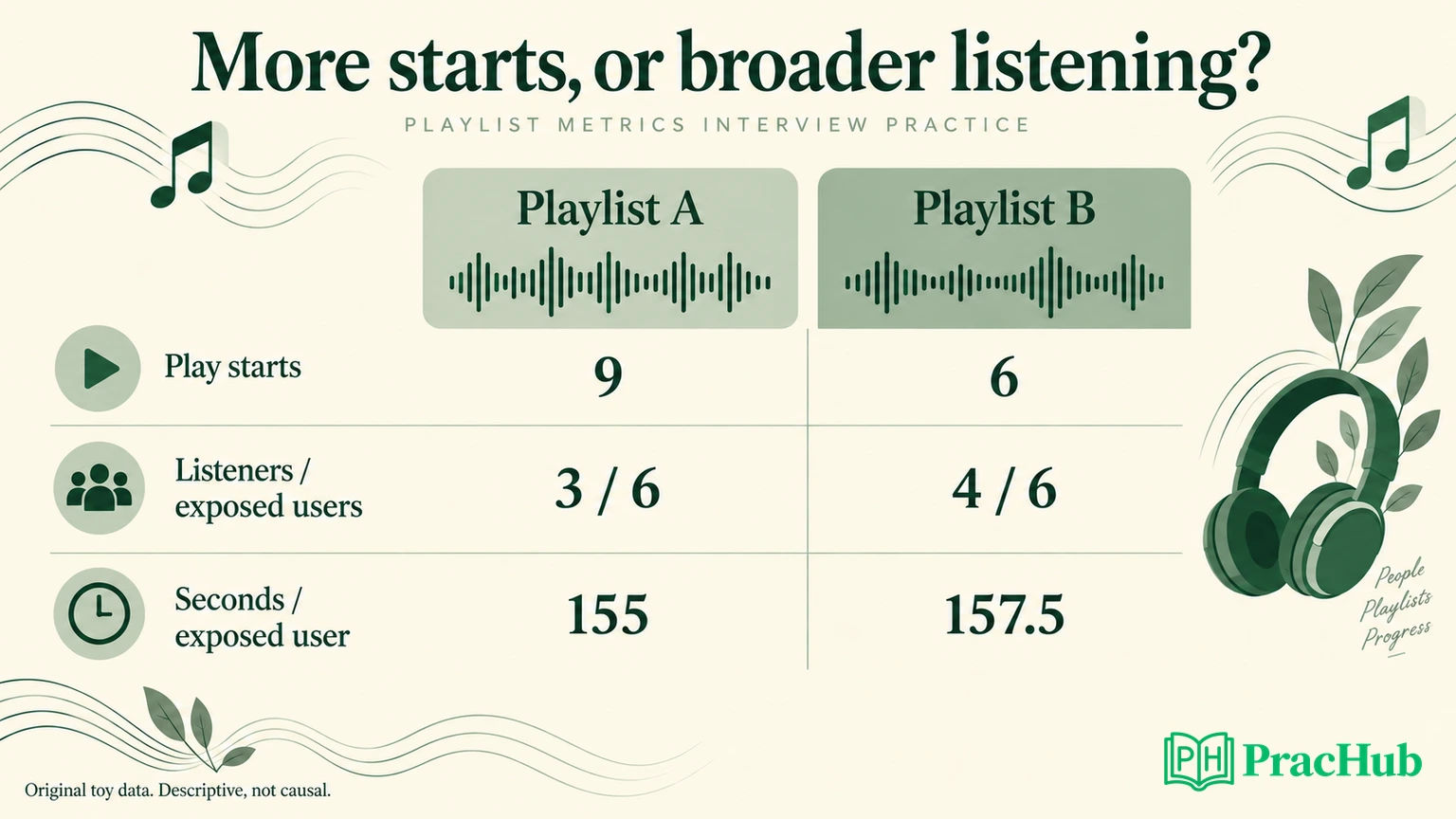
| Seconds per exposed user | 155.0 | 157.5 |
The fixture reconciles to 12 unique exposures and 15 valid matched playback starts. The exact exposure duplicate and exact playback duplicate do not increase the results. P98 contributes to A's starts and seconds but not its completion denominator.
A has 50% more playback starts than B: nine versus six. B reaches one more listener and produces slightly more listening per exposed user. A's starts are concentrated among three people, so its larger volume cannot be described as broader adoption.
These tiny counts are designed for hand checking, not hypothesis testing. Do not present the difference between 155 and 157.5 seconds as a statistically established improvement. It could change substantially with one additional listener or a different exposure mix.
Explain why completion is only a proxy
A high-completion rate can suggest that people remain with selected tracks, but interpretation depends on the listening context. Short tracks, familiar songs, background use, and fewer opportunities to skip can all change the metric without establishing better discovery.
The rate here is weighted by playback starts with known duration. A frequent listener contributes more observations than someone who starts one track. For a user-level experiment, do not pretend those starts are independent randomized people. Choose an analysis method consistent with the assignment and outcome unit.
Missing duration coverage is another diagnostic: A has metadata for eight of nine starts, while B has it for all six. If missingness is related to track type or a logging defect, the observed completion comparison may be selective. Fix or investigate that gap before treating it as a reliable quality signal.
For a discovery goal, you might additionally study saves, later voluntary returns, artist diversity, or explicit satisfaction. Define each carefully and distinguish data you have from data you wish you had. None of those outcomes can be inferred from this fixture.
Present two reasonable next steps from the same evidence
Option one: prioritize a controlled test of B. If the product objective is helping more exposed listeners engage, B's broader reach makes it a reasonable candidate for further testing. State that the current evidence is descriptive and that the listening-time difference is small.
Option two: investigate exposure and instrumentation first. If A and B were shown to different audience segments, positions, or times of day, their rates may reflect distribution rather than playlist quality. The unmatched play and missing duration also justify checking telemetry before allocating a larger experiment.
Both recommendations can be reasonable. The choice depends on whether the data contract and exposure comparability are trustworthy enough to support the next investment. “B wins” hides that decision; “B is the more promising test candidate under this objective” describes it accurately.
A one-page presentation can contain the objective, the three decisive metrics, the data exceptions, and the recommended next action. Keep the full SQL available for technical follow-up. Do not make an audience read every intermediate row to understand the recommendation.
Design the comparison you would want next
For a follow-up experiment, randomize eligible users before exposure and keep assignment stable. Compare the assigned populations using a prespecified outcome such as listening seconds per eligible user or a suitably defined engagement indicator. Retain people with zero listening in the primary analysis.
Do not condition the main experiment analysis on opening the playlist if assignment can affect whether people open it. Also distinguish the case's observed-exposure denominator from an experiment's assignment denominator. If the feature changes whether a card is displayed, exposure itself may be affected by treatment.
Prespecify the observation window, meaningful effect size, uncertainty method, and guardrails. Consider satisfaction, unwanted repetition, playback failures, and whether listening merely shifts away from other playlists. More listening on one surface does not automatically mean more total user value.
A technical follow-up might ask whether both playlists should have the same length or track mix. Explain the estimand: testing the whole product experience permits differences that are part of the treatment; isolating a ranking change may require holding other components constant. State which question the experiment answers.
Practice five related questions
These PracHub exercises cover adjacent data science, visualization, and recommendation skills. They are not a verified Spotify interview question set.
| PracHub question | Practice focus |
|---|---|
| Establish causality: commute playlist and driving speed | Challenge a causal story. |
| Design visualizations for streaming metrics | Choose a chart that preserves denominators. |
| Find recommended friend pairs by shared listening | Reason about listening joins and distinct users. |
| Design a Sequential Personalized Playlist Recommender | Connect recommendation choices to user context. |
| Defend an Experiment Decision and Its Incremental Impact | Explain a decision under uncertainty. |
Try the playlist causality exercise after presenting this case. Identify one alternative explanation for the observed difference and one measurement or design change that would help distinguish it.
Sources and Further Reading
- Spotify: Start your journey — official general hiring guidance.
- Aced, formerly Exponent: Spotify data scientist interview guide — third-party context, not a universal process specification.
- SQLite: Built-in aggregate functions — SQL behavior used in the worked example.
Comments (0)