SQL Query Optimization Interview Questions: EXPLAIN Plans, Joins, and Indexes
Quick Overview
Learn a practical SQL query optimization interview framework for reading EXPLAIN plans, diagnosing joins and cardinality, and choosing indexes with evidence.
A slow SQL query lands in front of you during an interview. The tempting answer is immediate: "add an index." That answer is sometimes right, but it skips the part interviewers actually care about: can you prove where the time goes, explain why the optimizer chose its plan, and make one change without breaking correctness?
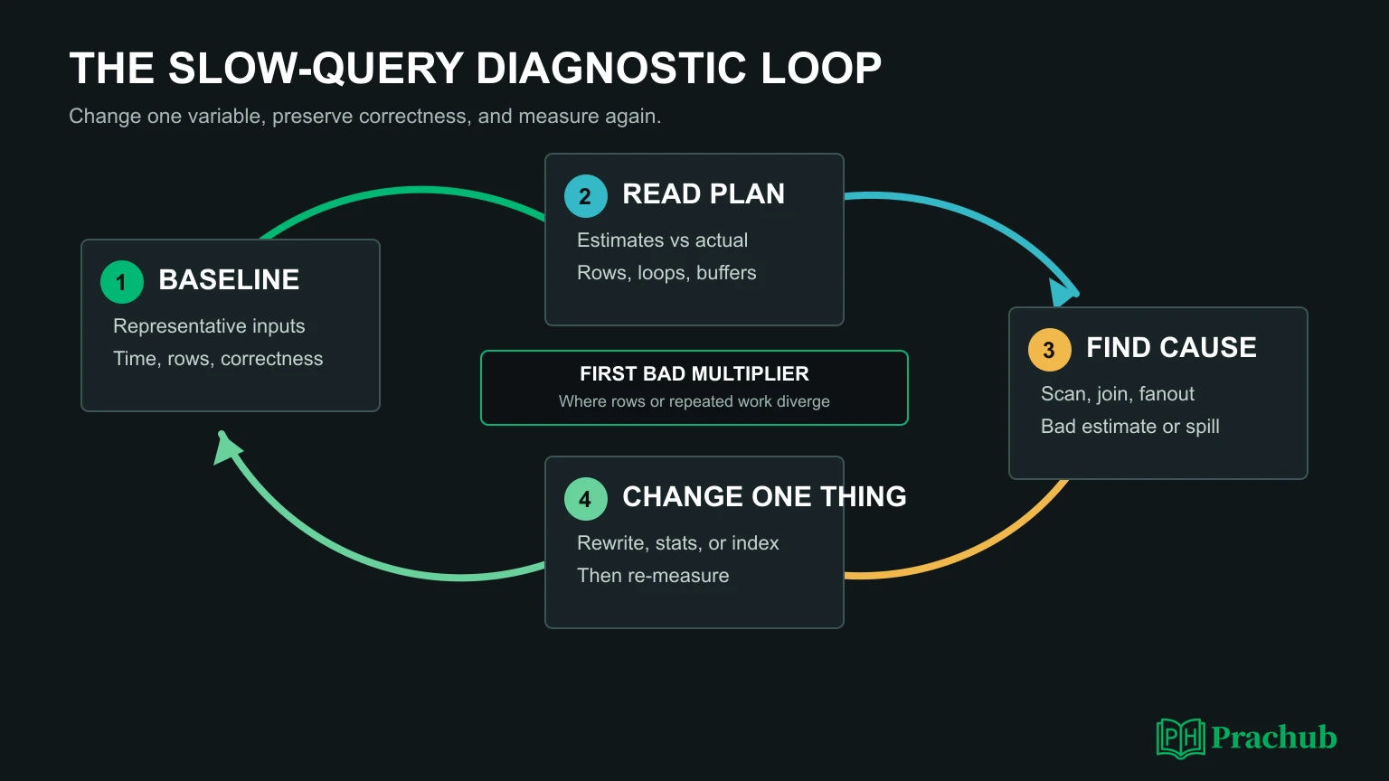
Strong candidates treat SQL query optimization as a diagnostic loop. They establish a baseline, inspect an execution plan, compare estimated and actual rows, trace joins and scans, change one bottleneck, and measure again. This guide shows that process with a realistic example and the signals hidden inside EXPLAIN.
To practice the query-writing side before adding performance constraints, work through PracHub's SQL interview questions. Then return to the same solutions and ask a second question: how would each query behave at ten million rows?

Quick answer: use a six-step optimization loop
A convincing interview answer follows a repeatable sequence:
- Confirm correctness and workload. Define the expected rows, data size, parameter values, latency target, and whether the query is read-heavy or write-sensitive.
- Measure a baseline. Record duration, rows returned, and representative inputs. A single warm-cache run is not a baseline.
- Read the actual plan. Start at the leaf scans and follow rows upward through joins, sorts, and aggregates.
- Find the first bad multiplier. Look for estimate errors, repeated inner loops, row explosion, discarded rows, and disk spills.
- Change one thing. Rewrite the query, refresh statistics, or add a justified index.
- Re-measure and recheck results. The optimized query must return the same answer and improve the target workload, not only one convenient input.
| Plan signal | What it may mean | Best first check |
|---|---|---|
| Estimated rows differ sharply from actual rows | Stale statistics, skew, correlated columns, or parameter sensitivity | Compare estimates at the earliest divergence and inspect data distribution |
| Inner node has many loops | Nested-loop work is being repeated | Multiply per-loop rows and time by loops |
| Many rows removed by a filter | The predicate is applied late or cannot drive access | Check predicate placement and sargability |
| Sort or hash uses disk | The input is too large for available memory | Reduce rows or width before increasing memory |
| Join output is far larger than either input | Many-to-many fanout or a missing join condition | Validate keys and expected cardinality before tuning |
| Sequential scan on a large table | Could be low selectivity, no useful index, or a non-sargable filter | Check rows needed versus rows scanned |
What interviewers are really scoring
Optimization questions test more than SQL syntax. Interviewers want to see whether you can connect data shape, access path, algorithm choice, and operational cost. A candidate who names every join type but never asks how many rows flow through the plan is reciting, not diagnosing.
They also watch how you handle uncertainty. You rarely know table sizes, distributions, existing indexes, or cache state at the start. Ask for them. If the interviewer cannot provide them, state assumptions and explain how a different assumption would change your decision.
Finally, protect correctness. Replacing a left join with an inner join, moving a predicate across an outer join, or pre-aggregating at the wrong grain can make a query fast and wrong. A strong answer identifies the result's grain and invariants before touching performance.
How to read an EXPLAIN plan without guessing
Read the tree from leaves to root
PostgreSQL documents an execution plan as a tree. Leaf nodes retrieve rows through sequential, index, or bitmap scans. Parent nodes join, sort, aggregate, or limit those rows. Start at the leaves and ask how many rows each node emits to its parent.
Do not read only the top line or chase the largest displayed cost. An upper node includes its children. The first lower node where row volume or work becomes unreasonable usually reveals the cause.
Separate cost, time, rows, and loops
Planner cost is expressed in optimizer units, not milliseconds. With EXPLAIN ANALYZE, actual time is measured runtime, while rows and loops describe how often work happened. In PostgreSQL, per-node actual values are averages per execution, so multiply them by loops to understand repeated work.
Estimated-versus-actual rows deserve special attention. If the optimizer expects 20 rows and receives 200,000, it may choose a nested loop that looked cheap on paper. That join is a symptom; the cardinality estimate that justified it may be the root cause.
Use actual plans carefully
EXPLAIN ANALYZE executes the statement in PostgreSQL and MySQL. For a read query in a safe test environment, that is usually what reveals true row counts and timing. For writes, expensive production queries, or side-effecting functions, use a controlled copy, an appropriate transaction strategy, or an estimated plan first.
SQL Server uses different tooling, but its actual plan is also generated after execution and includes runtime information and warnings. In an interview, name your assumed database instead of mixing operator terminology.
Scan nodes: a sequential scan is not automatically bad
A sequential scan can be the cheapest choice when a query needs much of a table or the table is small. An index lookup is not free: the engine must traverse the index and may perform scattered reads to fetch table rows. If 70 percent of a table qualifies, sequential access can beat thousands of random lookups.
An index scan is attractive for selective predicates, ordered access, and small result sets. A bitmap plan can combine index matches and fetch table pages in a more efficient order. An index-only scan may avoid heap reads when all required columns are available and the engine can verify row visibility without visiting the table.
Also inspect whether a condition is an access condition or a post-read filter. A predicate such as WHERE DATE(created_at) = '2026-08-01' may prevent a normal index on created_at from driving a range scan. A sargable range keeps the column unwrapped:
WHERE created_at >= DATE '2026-08-01'
  AND created_at <  DATE '2026-08-02'
Joins: explain the algorithm and the row flow
Nested loop
A nested loop reads outer rows and probes the inner input for each one. It can be excellent when the outer side is small and the inner side has a selective index. It becomes dangerous when the outer side is larger than estimated or the inner probe scans many rows each time.
Hash join
A hash join builds an in-memory hash table from one input and probes it with the other. It suits many equality joins, especially when a large portion of both inputs participates. Watch build-side size, row width, batches, and disk use; a hash that spills can lose much of its advantage.
Merge join
A merge join consumes inputs ordered by the join keys. It can be efficient for large sorted inputs or when indexes already provide the required order. If both sides require expensive sorts first, the total plan may be worse than a hash join.
There is no universally best join. Explain why the algorithm fits the inputs, then compare estimates with reality. Also check join fanout: joining multiple detail tables before aggregation can multiply rows and corrupt totals as well as performance.
Cardinality errors are often the real bottleneck
The optimizer chooses scans and joins from estimated row counts. Those estimates depend on statistics about table size, distinct values, common values, and distributions. Statistics are approximate and can become stale after significant data change.
Single-column statistics can also miss correlation. Suppose country = 'US' and state = 'CA' are treated as independent filters even though state strongly determines country. The combined estimate can be far from reality. PostgreSQL provides extended statistics for selected column groups because this problem cannot be solved by blindly increasing every statistics target.
Skew and parameter sensitivity matter too. A plan that works for a rare tenant can fail for the largest tenant. In an interview, ask whether the slow behavior occurs for all parameters, only certain customers, or only after a data-growth event. That question often separates a reusable fix from a benchmark trick.
Rewrite the query before reaching for another index
Imagine a report that returns each active customer's 2026 order count and payment total. The first draft joins raw orders and raw payments, then aggregates:
SELECT c.id,
       COUNT(o.id) AS order_count,
       SUM(p.amount) AS paid_amount
FROM customers c
JOIN orders o   ON o.customer_id = c.id
JOIN payments p ON p.order_id = o.id
WHERE c.status = 'active'
  AND EXTRACT(YEAR FROM o.created_at) = 2026
GROUP BY c.id;
Several risks are visible before seeing a plan. The function on created_at may block a range access path. Multiple payment rows can inflate COUNT(o.id). The query carries every matching payment row into the final aggregate.
A safer rewrite filters orders with a range and aggregates payments at the order grain before joining:
WITH paid_per_order AS (
  SELECT order_id, SUM(amount) AS paid_amount
  FROM payments
  WHERE status = 'settled'
  GROUP BY order_id
)
SELECT c.id,
       COUNT(*) AS order_count,
       COALESCE(SUM(p.paid_amount), 0) AS paid_amount
FROM customers c
JOIN orders o ON o.customer_id = c.id
LEFT JOIN paid_per_order p ON p.order_id = o.id
WHERE c.status = 'active'
  AND o.created_at >= TIMESTAMP '2026-01-01'
  AND o.created_at <  TIMESTAMP '2027-01-01'
GROUP BY c.id;
Now run the actual plan with representative data. Check whether the date range reduces orders early, whether payment aggregation spills, whether active-customer filtering is selective, and whether estimated rows match actual rows. Only then can you justify the next change.
When an index is the right fix
If the plan repeatedly needs a selective customer-and-date access path, an index such as orders(customer_id, created_at) may be useful. If the workload first filters a global date range and only later groups by customer, (created_at, customer_id) may fit better. Column order follows the real predicate and ordering pattern, not a memorized rule.
Every index adds storage and write maintenance, and a low-selectivity index may not be chosen. Covering more columns can reduce reads but increases index width. For the mechanics and write-tax discussion, use the companion database indexing interview guide; in this interview answer, keep the focus on evidence from the plan.
A good final statement sounds like this: "The plan shows a selective date-and-customer lookup repeated in the critical path, estimates are accurate, and the query rewrite still performs many table reads. I would test this composite index, compare buffers and latency before and after, and measure the insert/update cost before keeping it."
Practice SQL optimization questions on PracHub
These questions cover execution plans, scan reduction, index design, and large-table SQL. Use the stored role and prompt as practice context; they are not predictions of a specific future interview.
| PracHub question | Practice focus | Why it helps |
|---|---|---|
| Optimize SQL to Minimize Scans | CTEs, aggregation, and EXPLAIN | Forces you to prove that a rewrite reduces repeated table access. |
| Query an Indexed In-Memory Numeric Table | Index construction and candidate intersection | Connects indexing choices to preprocessing and query complexity. |
| Reason About Indexes, Kafka, and Database Locking | Access patterns, selectivity, and write cost | Builds the trade-off language expected in backend interviews. |
| Compute Paid Subscriber YoY Counts by Month | Large-table aggregation and anti-joins | Tests query structure, date ranges, and performance-aware correctness. |
A seven-day SQL optimization practice plan
| Day | Focus | What to do |
|---|---|---|
| Day 1 | Baselines | Time three queries with representative parameters and record rows returned. |
| Day 2 | Plan reading | Trace leaf scans to the root; label estimates, actual rows, loops, and buffers. |
| Day 3 | Join algorithms | Explain when nested-loop, hash, and merge joins fit different input sizes. |
| Day 4 | Cardinality | Find the first estimate error and propose a statistics or data-distribution check. |
| Day 5 | Query rewrites | Make predicates sargable and pre-aggregate one fanout-heavy query. |
| Day 6 | Index decisions | Design one composite index, then explain selectivity, coverage, and write cost. |
| Day 7 | Mock interview | Deliver the six-step loop aloud and defend one before-and-after plan. |
Frequently asked questions
Should I always use EXPLAIN ANALYZE?
No. It is valuable because it supplies actual runtime and row information, but it executes the statement. Use it where execution is safe. For risky writes or production-heavy queries, start with an estimated plan or a controlled environment.
Is an index scan always faster than a sequential scan?
No. A sequential scan can win when the table is small or the query needs a large fraction of its rows. Compare rows needed, pages read, ordering requirements, and random-access cost.
Which join type should I recommend in an interview?
Recommend the algorithm that fits the inputs. Nested loops favor a small outer side and cheap inner probes; hash joins fit many equality joins; merge joins benefit from ordered inputs. Then verify whether actual cardinalities support that choice.
What is the most important EXPLAIN number?
There is no single magic number. Start with the difference between estimated and actual rows, then inspect loops, rows removed, buffers, and spill information. Together they explain why the plan did more work than expected.
How do I prove an optimization worked?
Compare equivalent workloads before and after. Verify identical results, use representative parameters, repeat measurements, and inspect the new plan. Include the cost of extra indexes or memory rather than reporting latency alone.
Final takeaway
The best answer to SQL query optimization interview questions is not a bag of tricks. It is a disciplined explanation of what the query should return, how rows move through the plan, where estimates or work explode, and how one measured change fixes the cause.
Build that habit on PracHub's company-filterable SQL questions: solve the query, predict its plan, inspect the real plan, and defend the trade-offs. That turns SQL practice into the performance reasoning expected from data, backend, and senior engineering candidates.
Sources and Further Reading
- PostgreSQL: Using EXPLAIN
- PostgreSQL: Statistics Used by the Planner
- MySQL 8.4: EXPLAIN Statement
- Microsoft SQL Server: Display an Actual Execution Plan
Research note: This guide was checked on August 22, 2026. Operator names, statistics features, and plan output vary by database engine and version.
Comments (0)