A/B Testing And Statistical Inference

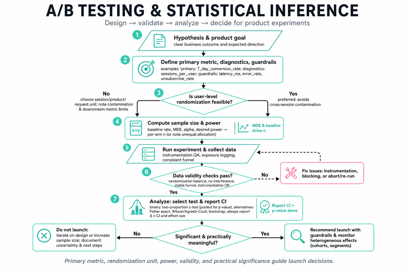
What's being tested

Interviewers are probing whether you can design, analyze, and explain online controlled experiments as a Data Scientist, not just run a canned significance test. You need to connect business/product goals to measurable outcomes, choose the right statistical test, check experiment validity, and make a launch recommendation under uncertainty. Amazon cares because small product changes at scale can move conversion_rate, CTR, revenue_per_visitor, delivery promises, or customer trust metrics, and a misleading experiment can cause expensive false launches or missed opportunities. Expect the interviewer to test both mechanics—sample size, confidence intervals, p-values—and judgment: metric selection, guardrails, heterogeneous effects, multiple comparisons, and whether the result is practically meaningful.

Core knowledge

• Randomized controlled trials estimate causal impact by assigning users, sessions, products, or requests to treatment and control before exposure. For most product experiments, user-level randomization is preferred because it avoids cross-session contamination and supports customer-level metrics like 7_day_conversion_rate.

• Metric design starts with a primary success metric, secondary diagnostic metrics, and guardrail metrics. Example: for a dashboard engagement test, primary could be weekly_active_users, secondary could be dashboard_sessions_per_user, and guardrails could include latency_ms, error_rate, unsubscribes, or downstream purchase_rate.

• Two-proportion z-tests are common for binary outcomes. For control conversion $\hat p_c=x_c/n_c$ and treatment conversion $\hat p_t=x_t/n_t$, the difference is $\Delta=\hat p_t-\hat p_c$. Under the null, use pooled rate $\hat p=(x_t+x_c)/(n_t+n_c)$ and standard error $SE_0=\sqrt{\hat p(1-\hat p)(1/n_t+1/n_c)}.$ Then $z=\Delta/SE_0$.

• Confidence intervals communicate estimation uncertainty better than p-values alone. For a binary metric difference, a common large-sample CI is $\Delta \pm z_{1-\alpha/2}\sqrt{\frac{\hat p_t(1-\hat p_t)}{n_t}+\frac{\hat p_c(1-\hat p_c)}{n_c}}.$ For small counts or rare events, mention Wilson, Agresti-Coull, Fisher’s exact test, or bootstrap as more robust alternatives.

• Power and sample size depend on baseline rate, minimum detectable effect, significance level, and desired power. For equal-sized two-arm binary tests, approximate per-arm sample size is $n \approx \frac{2\bar p(1-\bar p)(z_{1-\alpha/2}+z_{1-\beta})^2}{\delta^2},$ where $\delta$ is the absolute effect size. Smaller detectable effects require quadratically larger samples.

• Practical significance is different from statistical significance. At Amazon scale, a 0.03 percentage-point lift may be statistically significant but not worth shipping if it adds operational complexity, harms latency, or degrades a long-term trust metric. Always translate effect size into business/customer impact.

• Sample ratio mismatch is a validity check before interpreting treatment effects. If a planned 50/50 split produces 41/59 users, run a chi-square check against expected assignment counts. SRM often indicates assignment bugs, logging gaps, bot filtering asymmetry, eligibility mistakes, or exposure leakage.

• Unit of analysis must match the randomization unit. If randomization is by user but analysis treats page views as independent, p-values will be too small because within-user observations are correlated. Aggregate to user-level metrics or use cluster-robust standard errors when outcomes are repeated or clustered.

• Multiple testing inflates false positives when checking many metrics, segments, or variants. Bonferroni controls family-wise error with $\alpha/m$ but can be conservative; Benjamini-Hochberg controls false discovery rate. For interviews, say which comparisons were pre-registered versus exploratory.

• Variance reduction improves sensitivity without increasing traffic. CUPED uses pre-experiment behavior as a covariate: $Y_{adj}=Y-\theta(X-\bar X)$, where $X$ is a pre-period metric correlated with the outcome. It is especially useful for noisy continuous metrics like spend, sessions, or engagement time.

• Heterogeneous treatment effects should be handled carefully. Segment analysis by device, geography, new vs returning users, Prime vs non-Prime, or traffic source can reveal important effects, but these cuts are usually underpowered and subject to multiple comparison risk. Treat them as diagnostics unless pre-specified.

• Experiment duration should cover business cycles and avoid peeking-driven decisions. A 7-day test captures weekday/weekend behavior, but seasonality, promotions, novelty effects, and delayed conversions may require longer windows. If monitoring continuously, use sequential testing or alpha-spending rather than repeatedly checking naive p-values.

Worked example

For “Analyze an A/B test over last 7 days”, a strong candidate should start by clarifying the randomization unit, intended traffic split, eligibility criteria, primary metric, and whether the 7-day window is complete for delayed outcomes. Then state assumptions: users were randomized before exposure, assignment was stable, and each user is counted once for the primary binary conversion metric. The answer can be organized into four pillars: first, validate the experiment with sample sizes, exposure counts, and sample-ratio mismatch; second, compute treatment and control conversion rates plus absolute and relative lift; third, run statistical inference using a two-proportion z-test and confidence interval; fourth, inspect guardrails and important segments.

A good candidate would explicitly say they would not jump straight to “p < 0.05, ship it” before checking data validity and practical impact. For example, if treatment improves conversion_rate but worsens refund_rate, latency_ms, or customer complaints, the launch recommendation may change. One tradeoff to flag is whether to use all events or user-level aggregation: event-level analysis gives more rows but violates independence if the user is the randomized unit. The candidate should close with a decision framework: launch if the primary metric lift is statistically and practically meaningful, guardrails are neutral, SRM is clean, and effects are directionally consistent across major cohorts. If given more time, they should mention checking novelty effects, delayed conversions, pre-period balance, and whether the result holds under variance-reduced or cluster-robust analysis.

A second angle

For “Calculate A/B sample size, CI, decision rules”, the same ideas appear before the experiment rather than after it. The interviewer is testing whether you can design a test with enough power to detect a business-relevant effect, not reverse-engineer significance once the data arrives. You should ask for baseline conversion rate, minimum detectable effect, desired power, alpha, number of variants, and whether the metric is binary, continuous, ratio-based, or clustered. The framing shifts from “what happened?” to “what evidence will we require to make a decision?” A strong answer includes an explicit decision rule, such as: launch only if the 95% CI excludes zero, the lower bound exceeds the practical threshold, and guardrails remain within acceptable limits.

Common pitfalls

Pitfall: Treating p-value as the probability the null hypothesis is true.

A p-value is the probability of observing data at least as extreme as this result assuming the null is true. It is not $P(H_0 \mid data)$, and it does not measure effect size. A stronger answer pairs the p-value with a confidence interval, absolute lift, relative lift, and business impact.

Pitfall: Ignoring experiment validity checks and going straight to inference.

A tempting but weak answer is: “Control converted at 10%, treatment at 11%, p < 0.05, so ship.” Better: first check assignment ratio, exposure logging, duplicate users, bot/internal traffic, pre-period balance, metric denominator consistency, and whether the analysis unit matches randomization. Invalid randomization can make a beautiful confidence interval meaningless.

Pitfall: Overfitting the narrative to segments.

Candidates often slice by country, browser, customer tenure, and device until they find one impressive subgroup. That is exploratory analysis and should be labeled as such. The stronger version is to pre-specify key segments, correct or caveat multiple testing, and recommend follow-up experiments for surprising heterogeneous effects.

Connections

Interviewers may pivot from here to causal inference for non-randomized launches, including difference-in-differences, matching, regression adjustment, or instrumental variables. They may also connect to metric design, ranking/recommender evaluation, sequential testing, CUPED, or anomaly diagnosis when an experiment result conflicts with dashboard trends.

Further reading

• Trustworthy Online Controlled Experiments by Kohavi, Tang, and Xu — Practical treatment of experiment design, validity threats, metrics, and decision-making in large-scale online platforms.

• Controlled experiments on the web: survey and practical guide, Kohavi et al. — Seminal paper on online A/B testing pitfalls, ramping, metrics, and organizational practice.

• Improving the Sensitivity of Online Controlled Experiments by Deng, Xu, Kohavi, and Walker — Introduces CUPED-style variance reduction for online experiments.