LinkedIn Machine Learning Engineer Interview Prep Guide

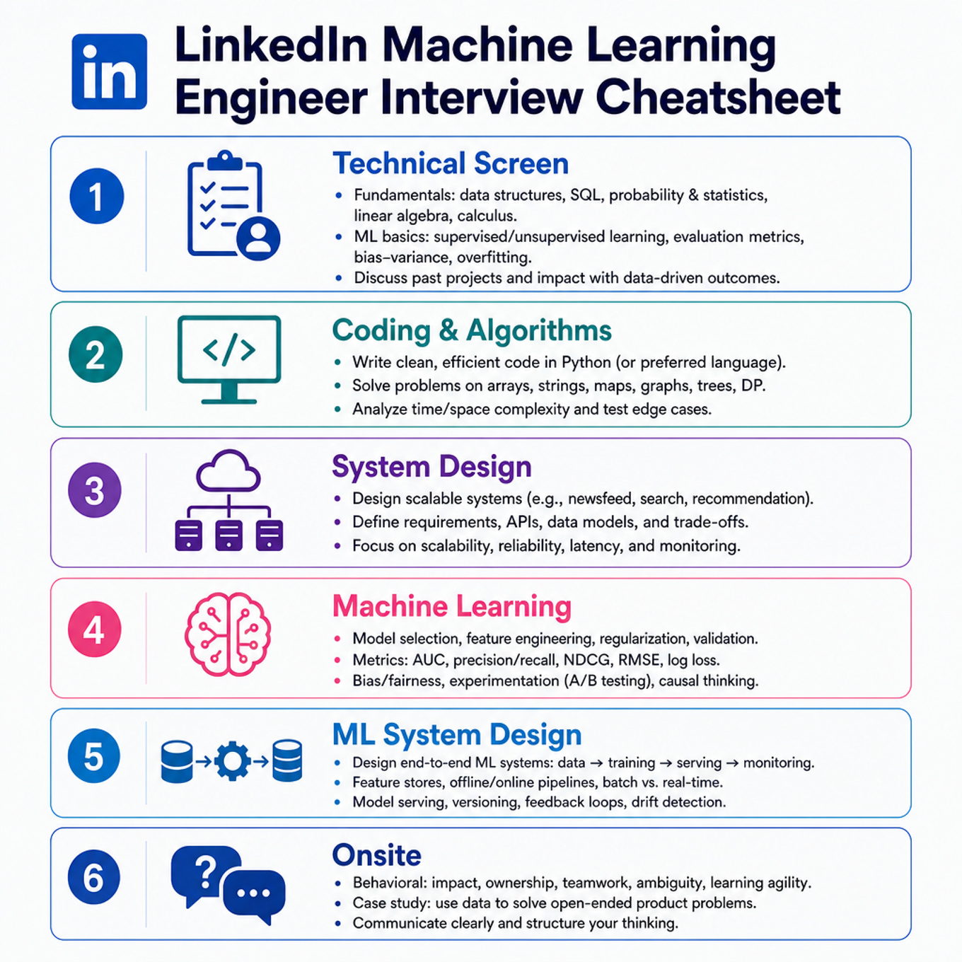
Focus most on LinkedIn-style recommendation/ranking, calibration, metrics experimentation, feature consistency, LLM adaptation, deployment safety, and phone-screen coding patterns because all self-ratings are 3/5, there are no solved-question signals, and your screen is in 5 days. No area is clearly strong from the signals, so graph BFS and interval sweep-line are kept brief because they were not selected as focus areas and missing concept ratings default to solid. The LinkedIn-specific emphasis is professional-graph recommendation systems, skill/entity inference, member-safe metrics, KV-backed stateful systems, and responsible AI for jobs, learning, and profile data. With less than a week, use this as a triage plan: prioritize Technical Screen sections first, then spend remaining time on onsite ML system design depth and senior-level tradeoff communication.

Technical Screen — 10 min

Coding & Algorithms

Focus area — You selected sliding-window and time-window counters; this is high-yield for phone-screen coding and metrics-style systems.

What's being tested

Candidates must demonstrate the ability to implement and reason about sliding-window algorithms and time-window counters over streams: correct incremental aggregation, memory/time tradeoffs, and robustness to timestamp issues. Interviewers probe whether you can pick the right data structure (queue, circular buffer, monotonic deque) and complexity bounds for high-throughput online counting or rate-detection tasks.

Patterns & templates

• Sliding-window (contiguous) — two-pointer expand/contract over arrays, O(n) time, O(1) extra space for fixed-size windows; handle empty-window edge cases.

• Fixed-size timestamp queue — collections.deque for append/pop timestamps, remove older-than-window, amortized O(1) per event, store counts or IDs.

• Bucketed time windows (circular buffer) — circular buffer of M buckets for window W, update bucket at ts % M, O(1) update; reset bucket on reuse.

• Monotonic deque for extrema — monotonic deque maintains candidate max/min in O(1) amortized per op, used for sliding max/min detection.

• Prefix-sum / difference arrays — precompute cumulative sums to answer many offline fixed-window queries in O(1) each; O(n) preprocessing.

• Approximate counters — CountMinSketch or exponential decay counters for low-memory, probabilistic counting; track error bounds vs memory.

• Time-decay / exponentially-weighted — use EWMA with factor α: $S_t = α x_t + (1−α) S_{t−1}$; constant memory for recency-weighted rates.

Common pitfalls

Pitfall: assuming strictly increasing timestamps — many streams have out-of-order or late events; you must decide tolerance or buffer/window adjustments.

Pitfall: reusing bucket without clearing — forget to store bucket's last-updated timestamp and you’ll mix old counts.

Pitfall: naive recompute per slide (O(k)) for large k — use incremental updates or monotonic structures to avoid TLE.

Practice these

The practice cards below cover the canonical variants — solve all of them and time yourself.

Practice questions

Technical Screen — 12 min

System Design

Focus area — You selected stateful data structures and KV stores; LinkedIn-scale systems often probe partitioning, replication, and hot-key tradeoffs.

What's being tested

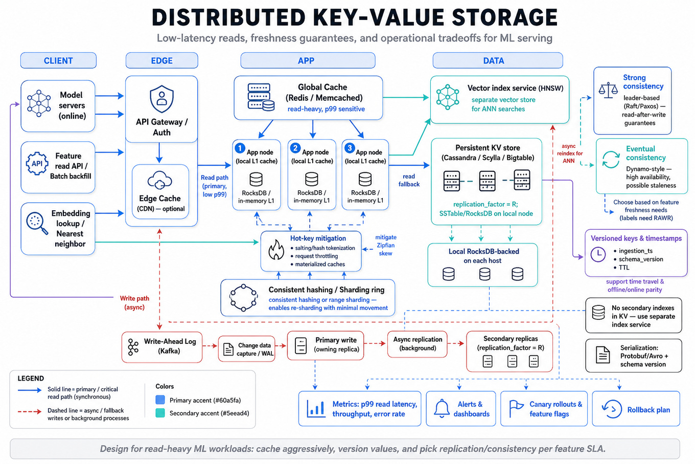
Interviewers are probing your ability to design a practical, reliable distributed key-value store that meets ML-serving needs: low-latency reads for features/embeddings, correctness of feature freshness (offline vs online parity), and operational trade-offs (consistency, replication, capacity, and monitoring). They want to see clear assumptions, an architecture addressing ML-specific access patterns, and how you reason about failures, rollback, and rollout for models that depend on this storage.

Core knowledge

• Workload characteristics: ML serving is typically read-heavy (reads:writes can be 100:1–1000:1), with tiny keys (IDs) and values that can be scalars, feature vectors, or embeddings (values 8B–1MB). Design to optimize for high read throughput and low tail latency (p99).

• Capacity math: total_storage_bytes = N_keys × avg_value_size × replication_factor. Include index/metadata overhead (~10–30%). Example: 100M keys × 1 KB × 3 → ~300 GB + overhead.

• Replication vs consistency: choose between strong consistency (leader-based, Raft/Paxos) and eventual consistency (Dynamo-style). ML-serving often tolerates slight staleness for features but requires read-after-write guarantees for label stores or online feature writes.

• Partitioning (sharding): use consistent hashing or range sharding to distribute keys and enable re-sharding with minimal movement. Hot-key mitigation (tokenization, hashing with salt) is essential for skew (Zipfian) access.

• Storage engines: for low-latency reads use in-memory stores (Redis, memcached), for large persistent KV use Cassandra/Scylla/Bigtable or local RocksDB backed services. Hybrid: local RocksDB + remote replication for cold storage.

• Indexing & lookup: avoid secondary indexes in simple KV stores; if you need attribute queries, use a separate index service. For embeddings, consider vector index (HNSW) separate from scalar feature KV.

• Serialization & schema: use compact binary formats (Protobuf, Avro) and include schema version and value TTL. Provide backwards-compatible readers for model rollouts.

• Feature freshness & time travel: support versioned keys or event-time stamped values to reproduce training-time feature views and ensure offline/online parity. Tag writes with ingestion timestamp and feature version.

• Caching & warmups: introduce a multi-tier cache (edge cache + local per-node cache). Tune TTLs per feature freshness guarantees; pre-warm caches during rollouts to avoid cold-start performance cliffs.

• Atomicity & multi-key updates: for multi-feature atomicity (all-or-none updates), either use transactional primitives (rare in distributed KV) or implement versioned bundles and read the latest consistent bundle.

• Monitoring & SLOs: instrument latency (median, p95, p99), error rate, cache hit-rate, eviction rate, and replication lag. Set SLOs for end-to-end ML request latency and degrade gracefully (fallback features/flags).

• Failure modes & recovery: handle node failure, network partition, and data corruption. Plan for repair (read-repair, anti-entropy), compaction, and backup/restore workflows. Consider how stale or missing features affect model outputs and user-facing metrics.

Worked example — "Design a distributed key-value store"

Start by clarifying scope and SLAs: ask about expected QPS, read/write ratio, p99 latency target, dataset size, and whether strong consistency is required for online writes. Declare assumptions: e.g., 10k QPS, 99.99% reads, 500M keys, p99 ≤ 10 ms, replication factor 3.

Organize the design into pillars: (1) partitioning & data placement with consistent hashing and hot-key mitigation; (2) replication & consistency model — choose leader replication with asynchronous replicas for reads, accept eventual consistency for features but enforce leader reads for label writes; (3) storage engine & caching — edge cache (CDN or local LRU) + persistent store (Cassandra or local RocksDB per node); (4) operational guarantees — monitoring, backups, schema versioning, and migration plan.

Flag tradeoff: choosing asynchronous replication reduces write latency but risks replication lag and stale features; mitigate by adding per-key version and letting model fetch the version or fall back to last-known-good. For rollout, stage migration by traffic percentage and pre-warm caches.

Close with next steps: if more time, design a concrete API (GET/PUT/GET-MANY), show failure-handling sequences (leader failover), sketch capacity diagrams, and write benchmarking scenarios to validate p99.

A second angle

Now assume the same store must host high-dimensional embeddings (512-d float vectors) for nearest-neighbor lookup in addition to scalar features. This changes constraints: value sizes increase (~2 KB per vector), storage and network cost rise, and read throughput per query may include bulk fetches (top-N lookups). You’d separate concerns: keep embeddings in a purpose-built vector store or a shard optimized for large values, enable compression (quantization, int8), and add batching APIs (GET_BATCH) to reduce RPC overhead. Also prioritize bandwidth-aware replication and prefetching; for model-serving, accept slightly higher latency for ANN searches but ensure deterministic fallbacks when the vector store is temporarily unavailable.

Common pitfalls

Pitfall: Designing for perfect consistency by default.
Assuming strong consistency everywhere increases latency and operational complexity; instead, pick per-data-class consistency based on how errors propagate to model outputs.

Pitfall: Ignoring tail latency sources.
Focusing on average latency hides p99 issues caused by GC, head-of-line blocking, and network spikes—these directly harm real-time model serving.

Pitfall: Treating feature store like a generic DB.
Using generic secondary indexes or cross-partition transactions for fast feature joins leads to brittle deployments. Prefer pre-joined feature bundles or versioned feature vectors for serving.

Connections

This topic commonly pivots to feature store design, online vs offline feature parity, or model serving architectures (e.g., embedding servers and model inference caches). Interviewers may also ask about monitoring-driven retraining pipelines (drift detection) or efficient bulk import for training offline replicas.

Further reading

• Dynamo: Amazon’s Highly Available Key-value Store — foundational tradeoffs between availability and consistency.

• Designing Data-Intensive Applications — chapters on replication, partitioning, and storage engines; practical for system tradeoffs relevant to ML serving.

Practice questions

• Metrics Monitoring And Experimentation (Focus) — covered in depth under Onsite below.

Technical Screen — 12 min

Machine Learning

• Transformer Internals And Scaling (Focus) — covered in depth under Onsite below.

• LLM Adaptation And PEFT (Focus) — covered in depth under Onsite below.

Technical Screen — 12 min

ML System Design

• Model Deployment Versioning And Safe Rollout (Focus) — covered in depth under Onsite below.

• GPU Scheduling And Resource Management (Focus) — covered in depth under Onsite below.

Onsite — 30 min

ML System Design

Focus area — You selected retrieval, candidate generation, reranking, and calibration; this is the core LinkedIn MLE system design surface.

What's being tested

Candidates must demonstrate practical design and engineering judgment for building low-latency, scalable recommendation and ranking pipelines: structuring candidate generation and reranking, ensuring online/offline feature parity, and handling feedback-driven learning (exploration/exploitation). Interviewers probe your ability to balance latency, freshness, and model quality while describing training/serving pipelines, evaluation metrics, and deployment/monitoring for iterative improvement. Expect to justify tradeoffs (batch vs. online learning, ANN memory vs. recall, exploration budget) from an MLE operational viewpoint.

Core knowledge

• Two-stage architecture: candidate generation reduces billions→thousands using heuristics/embedding nearest-neighbors; reranker scores candidates with rich features for final ordering and personalization.

• Feature freshness & consistency: use a feature store with both online (low-latency) and offline (batch) views; ensure training uses the same transformed features as serving to avoid training–serving skew.

• Embeddings & ANN: learn item/user embeddings (e.g., SGD or matrix factorization); use Faiss/product-quantization for ANN to serve nearest neighbors at scale—works for up to ~100M vectors with quantization.

• Latency budgets: set p99 SLO (e.g., <100ms for web, <20ms for mobile SDKs); push heavy computation offline or to candidate stage; reranker should be microseconds–milliseconds per candidate.

• Losses & objectives: choose objective aligned to business metric: binary cross-entropy for CTR, pairwise losses or LambdaRank for ranking (optimize NDCG). For multi-objective, scalarize or use constrained optimization (Lagrangian) to trade off watch-time vs. CTR.

• Cold-start: combine content-based features (metadata, category, textual embeddings) and popularity/recency heuristics; use meta-learning or warm-start embeddings via side features.

• Feedback-driven learning: apply contextual bandits for exploration-exploitation; evaluate policies with Inverse Propensity Scoring (IPS) where weight w = π(a|x)/π0(a|x), and prefer doubly-robust estimators to reduce variance.

• Offline evaluation vs. online metrics: use NDCG@k, AUC, calibration checks offline; validate with online metrics like CTR, session-duration, retention. Be explicit about metric-optimizing loss mismatch.

• Negative sampling & label delay: for implicit feedback, carefully design negative sampling and account for delayed labels (conversions) to avoid label bias; consider censoring or survival analysis if delays are long.

• Online learning & deployment: support incremental updates, periodic full retrains, and online updates for embeddings or shallow layers; use shadow serving and canary rollouts to validate model behavior before ramp.

• Drift detection & monitoring: monitor feature distributions (KL divergence), model output distribution, and online metric shifts; automate alerts for upstream feed changes or feature holidays.

• Privacy & fairness constraints: incorporate constraints (e.g., exposure caps) into ranking via post-processing (re-ranking) or constrained optimization, and log provenance for audits.

Worked example — "Design a real-time recommendation system"

First 30s: ask traffic/latency/memory SLOs, scale (DAU/items), acceptable exploration, and business objective (CTR, watch time, retention). State assumptions: 100M items, 50M DAU, p99 latency 100ms.

Skeleton answer pillars: (1) candidate generation (ANN on learned embeddings + time-decayed popularity and content filters), (2) feature-enriched reranker (gradient-boosted trees or small transformer using user/item/context features, cross-features), (3) training & feature pipeline (offline feature store, periodic retrain, online features via fast key-value store), (4) serving & rollout (low-latency microservice, shadow testing, canary).

Flag a tradeoff: ANN recall vs. latency—higher recall (larger probe count) improves candidate diversity but increases p99; prefer hybrid: static popularity + ANN top-K. Close with next steps: if more time, detail data schemas for features, show offline simulation of policy with IPS and design experiment allocation for safe exploration.

A second angle — "Design feedback-driven recommender"

This framing emphasizes online learning and exploration. Start by specifying the feedback loop latency and what counts as reward (click, watch-time normalized). Propose a contextual bandit layer on top of the baseline recommender to allocate exploration budget, instrument propensity logging for IPS/DR evaluation, and use Thompson Sampling or ε-greedy for initial exploration with decaying rates. Operational concerns: log full contexts and chosen-action propensities to enable unbiased offline evaluation; avoid catastrophic policy updates by constraining policy change per rollout. The core concepts (serving candidate/reranker separation, feature parity, monitoring) are the same but the priority shifts to safe online experimentation and reliable propensity bookkeeping.

Common pitfalls

Pitfall: Assuming offline metric improvement (e.g., lower training loss) directly transfers to online business metrics.
Many candidates optimize surrogate losses without addressing offline–online mismatch; explicitly discuss proxy-metric limitations and plan for online validation (shadow, canary).

Pitfall: Ignoring training–serving skew from missing/late features.
A tempting short answer is "use all signals"; stronger answers specify fallback features, imputation strategies, and tests that simulate production missingness during offline training.

Pitfall: Over-explaining infra details (e.g., Kafka partitions) instead of ML decisions.
Focus on model behavior, feature freshness, exploration policy, and monitoring; mention infrastructure only to justify feasibility and latencies.

Connections

Interviewers may pivot to causal inference (long-term value estimation and off-policy evaluation), CTR calibration and uplift modeling, or MLE topics like feature-store architecture and continuous deployment patterns (shadow traffic, canaries).

Further reading

• Recommender Systems Handbook (chapter on scalable training/serving) — comprehensive systems and algorithms overview.

• [Agarwal et al., “Counterfactual Evaluation for Recommender Systems”] — practical methods for IPS/doubly-robust policy evaluation.

Practice questions

Focus area — You selected deployment, versioning, safe rollout, batch inference, and serving; emphasize canaries, shadowing, rollback, and monitoring.

What's being tested

Interviewers are probing whether you can safely move models from training into production while maintaining reliability, observability, and rollbackability. Expect to demonstrate practical knowledge of model versioning, deployment patterns (canary/blue-green/shadow), production parity between offline and online features, and instrumentation for health and business metrics. Netflix cares because a bad rollout can harm availability, user experience, and long-running metrics; the interviewer wants assurance you can deploy without creating silent regressions.

Core knowledge

• Model registry and artifact immutability: use MLflow/internal registry to store artifacts, metadata, training dataset snapshot, training code hash and reproducible environment (Docker/SBOM). Immutable artifacts enable deterministic rollback.

• Semantic versioning for models: track major (backwards-incompatible input/schema), minor (performance/behavioural change), patch (bugfix). Enforce model signature checks (input schema, dtypes, feature names).

• Deployment patterns: blue-green (instant swap), canary (percent-based traffic ramp), shadow (mirror traffic for offline eval) and rolling (pods replaced gradually). Choose based on rollback speed vs. ability to observe business metrics.

• Online/offline parity: ensure feature computation in training matches serving via feature store (Feast) or shared transform libraries; run deterministic unit tests comparing offline predictions to online inference on identical inputs.

• Safeguards and gating: automatic checks for latency, error rate, prediction distribution drift, and primary business metric regressions; fail deployment when thresholds breached. Include p99 latency, request error-rate, and traffic saturation checks.

• A/B and sequential testing: coordinate with experimentation teams or implement lightweight holdout; for metric significance use confidence intervals $SE=\sqrt{\frac{p(1-p)}{n}}$ and consider sequential testing corrections (group-sequential or alpha-spending) for continuous rollouts.

• Drift detection: monitor feature population shifts (Population Stability Index, KL divergence), label distribution changes, and concept drift (ADWIN, MMD). Log inputs + predictions for delayed-label reconciliation.

• Logging and reconciliation: persist request features, model version, prediction, and trace id to durable store (sampled for cost) for replay and debugging; maintain label joins for offline accuracy checks as labels arrive.

• Resource and infra constraints: model size, memory, and CPU/GPU requirements affect autoscaling and cold-start. Consider quantization, batching, and caching for heavy models; measure throughput in RPS and latency percentiles.

• Rollout automation: CI/CD pipelines (ArgoCD, GitLab CI) should run contract tests, canary validation suites, smoke tests, and automated rollback triggers tied to monitored SLOs and business KPIs.

• Compatibility tests: include input-contract fuzzing, schema evolution tests, and backward/forward compatibility checks when features or encoders change (e.g., new categorical values).

• Security and privacy: ensure models and logs do not leak PII; apply access controls on model registry and artifacts, and sanitize feature logging.

Worked example — "Design a safe rollout for a new ranking model"

Frame it: ask clarifying questions first — what are the primary business metrics (CTR, watchtime), latency SLO, label delay, and available traffic for canary? Declare assumptions: labels arrive with X-hour delay; we can run a 5% canary. Skeleton answer pillars: (1) artifact/version/register model with metadata and signature tests; (2) pre-deploy smoke tests and offline holdout evaluation using the latest production traffic sample; (3) deploy a canary at 1% traffic with shadow mirroring to run on 100% for offline comparisons; (4) monitor infra (p99 latency, error-rate), prediction correctness proxies (cohort-level CTR predictors), and offline label-based metrics as labels appear; (5) automated gradual ramp to 25%/50%/100% with rollback on SLO breach or statistically significant negative delta using pre-defined thresholds. Tradeoff flagged: how long to wait for labels—short waits reduce rollout speed but long waits increase exposure. Close with next steps: "if more time, I'd add automated Bayesian sequential testing to speed safe decisions and a drift detector for feature shift to halt rollout early."

A second angle — "Model versioning and fast rollback in a multi-service system"

Here the constraint is many downstream services consume predictions or embeddings. Emphasize backward compatibility: ensure new model outputs (e.g., dim of embedding) remain compatible or provide adapter transforms. Use feature contracts and contract tests in CI to detect breaking changes. For rollback speed, separate model deployment from consumer rollout using a feature flag or routing at the API gateway so consumers can be toggled separately. Instrument cross-service tracing to detect cascading latency or scoring mismatches. This angle forces you to balance rapid rollback with the need for coordinated consumer changes and clarifies that model versioning must be discoverable and queryable by downstream services.

Common pitfalls

Pitfall: Assuming offline improvement implies production improvement. Offline metrics often overfit to training distribution; always validate with shadow runs and live canaries tied to business metrics.

Pitfall: Ignoring input-schema drift and hidden feature changes. A numeric-to-string upstream change can silently break preprocessing; add schema contracts and automated fuzz tests in CI.

Pitfall: Ramp decisions based only on infra metrics. Infrastructure stability is necessary but not sufficient — a model that increases latency may pass infra checks but still negatively affect retention or revenue; include business KPI monitoring and statistical testing in rollout gates.

Connections

Deployment and safe rollout often intersect with feature engineering / feature stores, model monitoring and observability, and CI/CD/infra automation. Interviewers may pivot to data-parity debugging, delayed-label evaluation pipelines, or scalability choices for serving (GPU vs CPU vs batch).

Further reading

• Continuous Delivery for Machine Learning (CD4ML) — ThoughtWorks — practical patterns for CI/CD applied to ML.

• MLflow Model Registry docs — implementation patterns for artifact/version management and model lifecycle.

Practice questions

Focus area — You explicitly selected GPU scheduling; senior AI interviews may test batching, utilization, quotas, autoscaling, and cost tradeoffs.

What's being tested

Interviewers are probing your practical knowledge of GPU resource tradeoffs and the scheduling strategies an ML Engineer uses to reliably run training and inference workloads at scale. Expect to justify choices that balance throughput, latency, cost, and isolation for multi-tenant ML workloads, and to show you can operationalize solutions (checkpointing, preemption, monitoring) rather than redesigning kernel schedulers or datacenter networks.

Core knowledge

• GPU memory (VRAM) versus model size: VRAM limits maximum model + optimizer state; use gradient accumulation or activation checkpointing when batch-size or model params exceed memory. Memory footprint ≈ params*4B (FP32) + optimizer states.

• Compute vs memory-bound: identify whether a model is compute-bound (SM utilization high, limited by FLOPS) or memory-bandwidth-bound (limited by DRAM/PCIe). Use nvidia-smi and DCGM metrics to measure SM utilization and memory throughput.

• Mixed precision: switching to FP16 / bfloat16 reduces memory and increases throughput via tensor cores; manage accumulation with a loss-scaling policy to avoid underflow. Typical speedups 1.5–3× depending on hardware.

• Data-parallel vs model-parallel: Data-parallel (DDP/NCCL AllReduce) is simplest for most models; switch to pipeline or tensor model parallelism when a single GPU cannot hold parameters. Communications scale: AllReduce cost ~ O(log N) for ring/allreduce algorithms but depends on network bandwidth.

• Interconnects: NVLink/NVSwitch and PCIe affect multi-GPU node performance; cross-node AllReduce is constrained by NIC bandwidth (e.g., 100 Gbps RoCE). Match topology-awareness in placement to reduce cross-node traffic.

• Scheduler primitives: key scheduler features include gang scheduling, device plugins (k8s GPU device plugin / NVIDIA GPU Operator), preemption, priority classes, and node selectors/taints for GPU types. Gang scheduling ensures all job tasks start together to avoid stragglers.

• Multi-tenancy & isolation: use MIG (A100+) for hardware partitioning, NVIDIA MPS for context multiplexing, or container-level limits for softer isolation. MIG gives stronger isolation and predictable VRAM/compute shares.

• Preemptible/spot instances & checkpointing: when using preemptible GPUs, design frequent checkpointing and incremental state saves; employ elastic/resumable training libraries (framework checkpoint + requeue logic). Checkpoint frequency trades off runtime overhead vs lost work.

• Fragmentation and packing: bin-packing increases utilization but may increase latency for large jobs; fragmentation metric = 1 − (sum idle_gpus / total_gpus). Defragment by backfill or allow preemption.

• Autoscaling & cost model: tie autoscaler to queued job depth and utilization thresholds (e.g., scale up if queued > k jobs or gpu_util < 0.7); compute cost per effective GPU-hour = raw_cost / (utilization). Optimize batch sizes and mixed precision to lower cost-per-step.

• Monitoring & SLOs: collect gpu_util, memory_used, memory_total, sm_efficiency, and job-level metrics (steps/sec, p95 latency). Define SLOs for throughput and job completion time; derive alerts from prometheus DCGM exporter.

Worked example — "Design a GPU scheduling strategy for a multi-tenant training cluster"

Frame: ask clarifying questions first — workload mix (short interactive jobs vs long batch training), SLA (fair-share or priority), toleration for preemption, allowed instance types (A100, V100), and whether checkpointing exists. Skeleton: (1) characterize workloads into classes (interactive, production retrain, hyperparameter sweep), (2) map classes to queues with priority and preemption rules, (3) choose scheduler primitives (gang scheduling for multi-node training, device plugin and node selectors for GPU types, MPS/MIG for small inference jobs), (4) pick autoscaling and checkpoint policy. Flag tradeoff: aggressive bin-packing and spot-instance usage improves cost but raises preemption and failure recovery complexity; prefer reserved capacity for high-priority training. Close by proposing measurable rollout: simulate scheduler using production traces, instrument DCGM and job completion metrics, and run a staged rollout with canary users. If more time: add fairness algorithms (DRF), scheduler simulator to tune backfill windows, and validate with adversarial workloads.

A second angle — "Optimize single-node multi‑GPU training throughput"

Here the focus shifts from scheduling to maximizing utilization on one machine. Start by profiling: overlap compute and communication by enabling NCCL asynchronous collectives and using gradient accumulation to increase compute per AllReduce. Use mixed precision to exploit tensor cores and reduce PCIe/NVLink pressure. If inter-GPU bandwidth is the bottleneck, prefer torch.distributed with nccl backend and enable /dev/shm staging for data loaders. Consider increasing per-GPU batch size until SM occupancy plateaus; if memory prevents this, use activation checkpointing. This framing emphasizes low-latency intra-node tricks rather than cluster-level allocation.

Common pitfalls

Pitfall: Optimizing for GPU count only. Many engineers request more GPUs without validating memory, interconnect, or IO, leading to poor utilization; always profile end-to-end (data loader → GPU compute → communication).

Pitfall: Ignoring preemption overhead. Assuming checkpointing is instantaneous underestimates lost work; quantify checkpoint time T_ckpt and requeue risk R to estimate expected wasted time = R * T_ckpt.

Pitfall: Overengineering scheduler features in interview. Propose a pragmatic incremental plan: classify workloads, implement priority queues, enable MIG/MPS, add checkpointing and monitoring, then iterate based on observed traces.

Connections

Interviewers often pivot to adjacent topics: distributed training algorithms (AllReduce vs parameter server), cost optimization (spot/commitment strategies), and data pipeline bottlenecks (sharded dataset serving, prefetching). Be ready to discuss how scheduling choices interact with dataset IO and model architecture.

Further reading

• NVIDIA MIG & Multi-Instance GPU — explains hardware partitioning and when to use it.

• NVIDIA Collective Communication Library (NCCL) Best Practices — guidance on tuning AllReduce and multi-GPU comms.

• Large Batch Training (Goyal et al., 2017) — useful for principled batch scaling and learning-rate schedules.

Practice questions

Onsite — 21 min

Machine Learning

Focus area — You selected ranking calibration, A/B testing, and metric design; no solved-question signal means this deserves extra review.

What's being tested

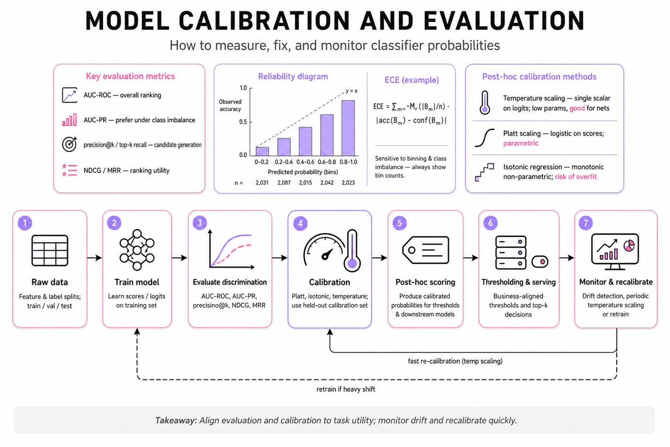
Candidates must show practical mastery of probability calibration and model evaluation for classifiers and rankers: how to measure calibrated probabilities, fix miscalibration, choose and justify evaluation metrics, and reason about offline→online gaps. LinkedIn cares because downstream systems (ranking, thresholding, personalization) rely on well-calibrated scores and appropriate evaluation to make safe, business-aligned decisions.

Core knowledge

• Calibration: the property that reported probability p means the event occurs ≈p fraction of the time; essential when scores drive thresholds, costs, or downstream probabilistic models.

• Reliability diagram: plot observed accuracy vs predicted confidence across bins; use equal-width or equal-frequency bins and show sample counts per bin to avoid misleading visuals.

• Expected Calibration Error (ECE): common scalar summary: $\text{ECE}=\sum_{m=1}^M\frac{|B_m|}{n}\big|\text{acc}(B_m)-\text{conf}(B_m)\big|$ where bins B_m partition examples; sensitive to binning choice and class imbalance.

• Brier score and log-loss: Brier = $\frac{1}{n}\sum_{i}(p_i-y_i)^2$; log-loss penalizes confident wrong predictions more; both combine calibration + discrimination.

• Discrimination metrics: AUC-ROC, AUC-PR (prefer PR under heavy class imbalance), precision@k, NDCG, MRR for ranking — pick metrics aligned to task utility (e.g., top-k recall for candidate generation).

• Post-hoc calibration methods: Platt scaling (logistic regression on scores), isotonic regression (monotonic non-parametric mapping; risk of overfitting), temperature scaling (single scalar T on logits; minimal params, good for modern nets). Use a held-out validation/calibration set, never the training set.

• Multi-class calibration: apply temperature or vector/matrix scaling to logits; can use one-vs-rest Platt for large label sets; measure per-class ECE or class-weighted ECE.

• Data shift and recalibration: calibration can break under covariate or label shift. Monitor distribution drift and recalibrate periodically; prefer fast methods like temperature scaling for online re-calibration.

• Practical tooling: sklearn.calibration.CalibratedClassifierCV for Platt/isotonic; scikit-learn, PyTorch/TensorFlow for logits and temperature scaling; Prometheus/Grafana or custom metrics to track calibration drift in production.

• Evaluation design: use time-based splits for temporal data, stratified sampling for rare classes, and cross-validation for small datasets; compute confidence intervals via bootstrapping for metrics like ECE or AUC.

• Threshold selection: determine thresholds by optimizing task-specific utility (F1, cost-weighted loss, business KPIs) on validation data and test robustness under shifted distributions.

• Ranking vs scoring: when converting ranking scores to probabilities, validate calibration against implicit feedback biases (exposure, position); consider counterfactual evaluation (IPS) if evaluating causal effects.

Worked example — "Answer practical ML foundations questions"

Frame: ask which downstream decisions use the probabilities, class imbalance severity, and whether calibration must hold across cohorts (geography, device). Declare assumptions: offline labeled validation set exists and distribution approximates production. Structure answer into three pillars: (1) diagnostic — compute reliability diagram, ECE, Brier, and AUC-PR; (2) remediation — try temperature scaling first (low-risk), then Platt or isotonic regression if non-monotonic errors persist; (3) deployment & monitoring — validate on held-out set, push to canary traffic, track online calibration metrics and trigger recalibration. A key tradeoff: isotonic regression can overfit with small calibration sets but models arbitrary monotone distortions; temperature scaling is robust with small sets but only fixes "softness" of logits. Close by saying: "If I had more time I'd run per-cohort ECE, test matrix-scaling for large multiclass error, and simulate label shift to stress-test recalibration frequency."

A second angle — "Design LinkedIn Learning course recommendations"

Here the same calibration and evaluation concepts focus on ranking and conversion modeling. You'd predict click/engagement probabilities for personalized ranking; require calibrated scores for fair exploration and downstream decision policy (e.g., allocate impressions). Diagnostics: compute calibration conditional on position/exposure to control for position bias, and evaluate NDCG or precision@k alongside ECE. For remediation, fit propensity-corrected calibration (re-weight examples by exposure IPS) or calibrate on logged-exposure data. Operational constraints (latency, model size) push toward lightweight calibrators like temperature scaling served with the model, and monitoring must detect shifts in content tastes so you can retrain and recalibrate pipelines.

Common pitfalls

Pitfall: Reporting low ECE as "good" without checking class imbalance.

ECE can be small when most mass is on a well-calibrated majority class; compute per-class or class-weighted ECE and examine reliability diagrams.

Pitfall: Calibrating on the training set or using the test set for tuning.

Always use a separate calibration/validation set to fit Platt/isotonic/temperature parameters; otherwise calibration will be overoptimistic.

Pitfall: Equating high AUC with good probabilities.

A model with excellent ranking (AUC) can be badly calibrated; decide early whether ranking or well-calibrated probabilities drive product decisions and optimize accordingly.

Connections

Interviewers often pivot to uncertainty quantification (Bayesian nets, MC-dropout), online monitoring & drift detection (dataset shift alarms, retraining triggers), or experiment design (A/B test sensitivity when using thresholds). Be prepared to connect calibration fixes to deployment mechanics and monitoring.

Further reading

• On Calibration of Modern Neural Networks — Guo et al., 2017 — seminal paper showing temperature scaling effectiveness.

• Predicting Good Probabilities — Niculescu-Mizil & Caruana, 2005 — empirical comparison of calibration methods.

Practice questions

Focus area — You explicitly selected transformer internals and have a senior AI phone screen in 5 days; prioritize attention, scaling, and inference costs.

What's being tested

Interviewers are probing whether you can design, scale, and operate Transformer training and inference for production — balancing compute, memory, cost, and latency. Expect to justify choices among data parallelism, model parallelism, optimizer memory-reduction techniques, precision formats, and inference optimizations. They also want you to reason about tradeoffs (time-to-train, p99 latency, cost) and failure modes relevant to production ML pipelines.

Core knowledge

• Transformer architecture basics: self-attention cost is $O(L^2·d)$ for sequence length $L$ and hidden dim $d$; attention dominates memory for long sequences, so sequence-length scaling is the first cost lever.

• Data parallelism: replicate parameters on each device, shard minibatches; communication is typically gradient synchronization via AllReduce (NCCL). Effective batch size = batch_per_gpu × num_gpus × grad_accum_steps; remember learning-rate scaling rules.

• Model parallelism: split parameters across devices. Two common types: tensor (operator) parallelism (e.g., Megatron-LM) slices large matrices across GPUs; pipeline parallelism splits layers into stages and streams micro-batches to fill bubbles. Combine with data parallelism for hybrid scaling.

• Memory-saving techniques: activation checkpointing (recompute activations on backward pass), optimizer-state sharding (ZeRO stages), and offloading (CPU or NVMe) trade memory for extra compute/IO. ZeRO Stage 1: shard optimizer states; Stage 2: shard gradients; Stage 3: shard parameters (no replication).

• Mixed precision: using FP16/bfloat16 with automatic mixed precision (AMP) reduces memory and increases throughput; requires loss scaling to avoid underflow and gradient blowup. Watch for non-determinism and numeric instability.

• Gradient accumulation and micro-batching allow larger effective batch sizes on limited hardware but increase staleness of optimizer state and wall-clock time per step.

• Communication bottlenecks: measure compute-to-communication ratio; ring AllReduce complexity is $O(n)$ bandwidth per node; network bandwidth (Infiniband, RoCE) and topology (fat-tree vs hierarchical) heavily influence scalability.

• Checkpointing & fault tolerance: balance checkpoint frequency vs storage; use incremental or sharded checkpoints (e.g., FSDP) to reduce I/O; know restart time implications for preemptible instances.

• Inference optimizations: KV-cache for autoregressive decoding, batched tokenization, beam search cost ~ beam_size×per-token cost, and model sharding for large models. Use model quantization (dynamic/static, per-channel) and distillation to cut latency/cost.

• Scaling laws: empirical law: loss decreases as a power-law with compute/model size (Kaplan et al.); this informs whether to scale model size vs dataset size vs compute investment. There are diminishing returns — quantify with FLOPs and dataset size.

• Monitoring & SLOs: key metrics include p50/p95/p99 latency, throughput (tokens/sec), model quality (e.g., perplexity for LM), and data/model drift (feature distribution shifts, embedding cosine similarity). Instrument cache hit rate for KV caches and host memory pressure.

Tip: use DeepSpeed/FSDP for out-of-the-box ZeRO-like sharding; benchmark on representative sequence lengths and payloads (not toy inputs).

Worked example — “Design a training pipeline to train a 10B-parameter Transformer on an 8-GPU cluster”

Frame: ask about target dataset size, desired time-to-train, budget, and whether GPUs have >40GB. Assume 8×A100 40GB and a large web-text dataset. Organize answer into (1) memory & parallelism plan, (2) optimizer/precision choices, (3) data/IO and checkpointing, (4) monitoring and rollback. Recommend hybrid approach: use tensor parallelism (split large layers across 2 GPUs) + data parallelism across the remaining factor; or use ZeRO Stage 2/3 via DeepSpeed/FSDP to fit on 8 GPUs. Use mixed precision (FP16) with dynamic loss scaling and activation checkpointing to reduce activations memory. Set effective batch size from throughput experiments, and apply linear LR scaling with warmup. Flag tradeoff: pipeline/tensor parallelism reduces memory per device but increases cross-device communication and latency; check compute-to-communication ratio and network speeds. Close by saying: if more time, I'd prototype two configs (ZeRO vs tensor+pipeline) with microbenchmarks on representative sequence length and instrument memory/comm breakdowns.

A second angle — “Serve a 2B-parameter Transformer for sub-100ms p99 conversational responses”

Frame: constraints shift from batch throughput to latency and cost. Key pillars: (1) model compression (quantization to 8-bit or 4-bit, and possibly distillation to a smaller model), (2) serving architecture (sharded model with fast interconnect or replicate smaller models for single-node inference), (3) request batching strategies (token-level batching, async decode), and (4) caching and request routing (hot-session KV cache). Tradeoffs: aggressive quantization may slightly reduce quality; sharding reduces memory per machine but adds cross-host latency for each token. If p99 is strict, favor replicated smaller models per machine with mmap-backed weights and efficient token batching. Add monitoring for tail latencies and cache hit rate. With more time, plan A/B on quality vs latency using offline evaluation (perplexity/utility) and small online experiment.

Common pitfalls

Pitfall: optimizing only for throughput and ignoring tail latency. A setup that maximizes tokens/sec can still fail SLOs if p99 is high due to cross-host communication or blocking IO.

Pitfall: scaling batch size without re-tuning learning-rate schedule. Applying linear LR scaling without proper warmup or warmup length change often causes divergence or worse generalization.

Pitfall: assuming mixed precision automatically works. Not handling NaN via loss scaling, or missing ops that require FP32 (layernorm accumulators, softmax reductions), leads to silent numerical errors.

Connections

Adjacent pivots interviewers often make: distributed systems networking (bandwidth/topology implications) and model evaluation/experiment design (how quality tradeoffs affect user metrics). Be ready to hand off to a Software Engineer for low-level network tuning or to a Data Scientist for experimental metric design.

Further reading

• Scaling Laws for Neural Language Models (Kaplan et al.) — empirical guidance on compute/model/dataset tradeoffs.

• ZeRO & DeepSpeed paper/blog — practical memory sharding strategies and system design for large models.

• Megatron-LM paper — details on tensor and pipeline parallelism for large Transformer training.

Practice questions

Focus area — You explicitly selected LLM adaptation and PEFT; prepare LoRA, prompt tuning, fine-tuning tradeoffs, and evaluation.

What's being tested

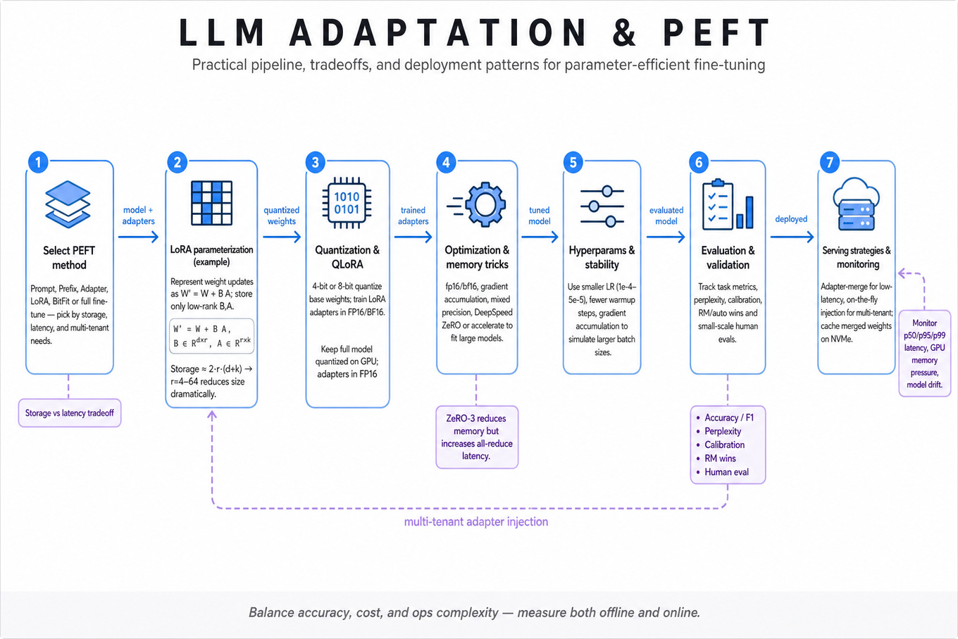
Interviewers are checking whether you can practically adapt large language models for production use: choose the right parameter-efficient fine-tuning (PEFT) method, design a training pipeline that fits compute and latency constraints, and evaluate tradeoffs between accuracy, cost, and operational complexity. They want to see system-level thinking (memory, throughput, serving strategy), empirical tuning (hyperparameters and validation), and monitoring/deployment practices that keep offline and online behavior aligned.

Core knowledge

• PEFT taxonomy — know common classes: prompt tuning, prefix tuning, adapter layers, LoRA, BitFit, and full fine-tuning; each differs in which parameters are updated and stored versus frozen.

• LoRA parameterization — represent weight updates as $W' = W + BA$ with $B∈R^{d×r}, A∈R^{r×k}$; storage scales with $2·r·(d+k)$, so small $r$ (e.g., 4–64) yields large savings.

• Quantization fundamentals — 8-bit and 4-bit inference reduce memory and bandwidth; bitsandbytes and transformers enable 8/4-bit weights and optimizer state; quantization may increase perplexity and require calibration.

• QLoRA pattern — combine 4-bit quantization with LoRA-style updates so full model stays quantized on GPU while low-rank adapters are trained in FP16/BF16; reduces memory enough to fine-tune 30B+ models on single GPUs.

• Optimization & memory tricks — use fp16/bf16, gradient accumulation, mixed precision, DeepSpeed ZeRO stages (especially ZeRO-3) or accelerate to distribute state; tradeoff: ZeRO reduces memory at cost of all-reduce and latency.

• Hyperparameter heuristics for PEFT — use smaller learning rates (e.g., $1e-4–5e-5$) and fewer warmup steps than full-tuning; batch size impacts stability—use gradient accumulation to simulate larger batches.

• Evaluation metrics & validation — for instruction-tuning track task-specific metrics (accuracy, F1), plus perplexity and calibration (confidence vs accuracy); for conversational/instruction models include automated reward-model wins and small-scale human evals.

• Serving strategies — adapter-merge (merge LoRA into base) for low-latency single-tenant inference; on-the-fly adapter injection for multi-tenant; cache merged weights in fast storage (NVMe) to avoid repeated merges.

• Operational monitoring — monitor latency $p_{50}/p_{95}/p_{99}$, GPU memory pressure, token throughput, distributional drift (embedding distance, KL divergence, change in perplexity) and user-facing metrics (error rate, fallback rate).

• Model lifecycle & storage — store many small adapter artifacts instead of multiple full checkpoints; version adapters with metadata (base model hash, tokenizer, quantization bits, LoRA rank, dataset snapshot).

• Failure modes & safety — PEFT can underfit domain shifts or maintain old behavior (catastrophic forgetting less likely than full fine-tuning); watch hallucinations and calibration shifts after adaptation.

• Cost/benefit calculus — estimate cost by memory footprints and GPU-hours: adapting with LoRA + 4-bit quantization often reduces GPU memory ~3–10× compared to full FP16 fine-tuning, enabling cheaper experiments and faster iteration.

Worked example

Problem framing: "Adapt a 34B LLM to a new enterprise domain with 10k labeled pairs and tight latency." First ask clarifying questions: required latency and throughput, whether multi-tenant adapters are needed, available GPU memory, and evaluation success metrics. Skeleton plan: (1) choose QLoRA + LoRA so the base model remains 4-bit quantized and only low-rank adapters are trained; (2) preprocess and split data for SFT, hold out a validation set and a small human-eval set; (3) pick LoRA rank $r$ (start 8–16), bf16 training, gradient accumulation, and DeepSpeed/accelerate for training stability; (4) evaluate with task metrics, perplexity, and a small instruction-following human check. Tradeoff flagged: increasing $r$ raises adaptation capacity but increases latency and storage per adapter—start small and scale $r$ based on validation gains. Closing: "If I had more time, I'd run a grid over $r$ and learning rate, do adapter-merge experiments for serving, and run small-scale RLHF or reward-model tuning to align outputs to business preferences."

A second angle

Consider a different constraint: "support thousands of customers each needing a personalized adapter, with strict per-request latency." The same PEFT concept applies but operational constraints dominate. Instead of merging adapters into full models for each customer (storage and load time explosion), use a runtime adapter-injection server that caches the most-active merged weights in GPU memory and serves others from an on-disk merged store with async warm-up. Batch requests by adapter id to amortize merge overhead. Here the adaptation design prioritizes adapter storage efficiency (LoRA with small $r$, compressed adapters) and a cache eviction policy based on QPS per tenant rather than maximizing per-adapter accuracy.

Common pitfalls

Pitfall: Underestimating memory/perf constraints — assume LoRA automatically fits your device; you must account for quantized base weights, optimizer state, and activation memory, or you'll OOM during training.

Pitfall: Using full-finetuning hyperparameters — PEFT changes effective parameter scale; use lower learning rates and monitor validation loss closely to avoid divergence or catastrophic overfitting to small datasets.

Pitfall: Ignoring serving complexity — proposing many small adapters without a serving plan leads to high cold-start latency and increased operational cost; articulate caching, merge-on-deploy, or multi-tenant injection strategies.

Connections

Interviewers may pivot to model compression & quantization (practical tradeoffs and tools), training infra (ZeRO, pipeline parallelism), or evaluation & monitoring (automated vs human evaluation, calibration, and drift detection).

Further reading

• LoRA paper (Hu et al.) — foundational low-rank adaptation technique and math rationale.

• Hugging Face PEFT library docs — practical examples for LoRA, adapters, and integration with transformers.

• QLoRA blog/post by Hugging Face — how 4-bit quantization + LoRA enables fine-tuning of very large models on commodity GPUs.

Practice questions

Onsite — 6 min

System Design

Focus area — You selected A/B testing and metric design, and viewed system design content without solved signals; emphasize decision-quality metrics.

What's being tested

Interviewers are checking your ability to define, instrument, monitor, and experiment on ML-driven metrics so models behave safely and improve reliably in production. Expect to show judgment about metric selection, statistical validity for A/B test designs, drift detection, alerting strategies, and how monitoring ties into model rollout and rollback. LinkedIn cares because model regressions or silent drift directly affect member experience and business outcomes; the engineer must reliably detect, diagnose, and act.

Core knowledge

• Metric taxonomy: classify metrics as primary business (DAU, revenue-per-user), model quality (CTR, precision@k, NDCG), guardrail (latency, error-rate), and diagnostic (feature distributions, cohort breakdowns).

• Experiment statistics: know hypothesis tests, type-I/II errors, $p$-values, and that the required sample size for a continuous metric is $n\approx\left(\frac{Z_{1-\alpha/2}+Z_{power}}{\Delta/\sigma}\right)^2$ where $\Delta$ is detectable effect and $\sigma$ is stddev.

• Multiple comparisons & FDR: when monitoring many metrics or segments use Benjamini–Hochberg to control False Discovery Rate or Bonferroni for conservative familywise control; naive per-metric $p$-values inflate false positives.

• Sequential testing: understand fixed-horizon vs sequential tests (alpha-spending, SPRT, Bayesian), and that naïve peeking invalidates $p$-values; use proper corrections or sequential-safe methods for long-running experiments.

• Sample Ratio Mismatch (SRM): always validate randomization by checking assignment ratios; SRM indicates logging, instrumentation, or bucketing bugs—an early guardrail before analyzing metrics.

• Drift detection: separate population drift (feature distribution) from concept drift (label relationship). Use KS-test, Population Stability Index (PSI), KL divergence, or model prediction-shift statistics; PSI > 0.1 is moderate drift.

• Anomaly detection: baseline algorithms: rolling z-score, EWMA, CUSUM for small persistent shifts, and seasonality-aware decompositions; tune sensitivity to balance detection vs alert fatigue.

• Attribution & exposure logging: for correct experiment evaluation log deterministic exposure events and impressions, not just clicks; without exposures you cannot compute accurate denominators or apply inverse-propensity weighting.

• Offline vs online parity: track feature freshness, training-serving skew, and reproducing offline metrics; keep a short feedback loop (canary + shadow) to validate online behavior matches offline expectations.

• Alerting strategy: tier alerts by severity (SLO breach, metric drift, experiment regression) and provide automated triage (top contributing segments, recent model versions, feature changes) to reduce toil.

• Power & minimum detectable effect (MDE): specify MDE before running experiments; small MDE implies very large sample sizes—prioritize metrics that matter and aggregate thoughtfully (daily vs weekly).

• Cohort & segmentation: predefine cohorts for diagnostic drilling (device, locale, new vs returning); beware slicing small cohorts which raises variance and false positives; use hierarchical testing to control errors.

Worked example — Design a scalable metrics monitoring system

First 30s: clarify scale (requests/sec, number of metrics), latency needs (real-time vs daily), and ownership (who acts on alerts). Declare assumptions: millions of users, both streaming and daily aggregated metrics, and A/B test experiments run continuously.

Skeleton pillars to communicate:

1. Metric contract & instrumentation: a canonical metrics registry with definitions, ownership, and deterministic exposure logging to ensure correct denominators.

2. Aggregation layer: two paths — low-latency streaming summaries for p99/real-time alerts and batch daily aggregates for stable metrics and experiments.

3. Detection & alerting: combine statistical tests (SRM checks, sequential tests) with anomaly detectors (EWMA, CUSUM) and tiered alerting (auto-mitigate minor alarms; page SRE for SLO breaches).

4. Experiment integration: tie metrics to assignment token, track treatment/control, run pre-specified analysis pipelines with multiplicity control and power checks.

5. Operational tooling: dashboards, automatic diagnostic drilldowns (top-k segments, change in top features), runbooks and canary rollback hooks.

Key tradeoff: sensitivity vs alert fatigue — choose higher thresholds or aggregate windows to reduce false positives, but provide fast detection for regressions in critical metrics. Close by saying: if more time, I’d sketch event schema, select specific algorithms for the streaming path, and prototype SRM and FDR workflows end-to-end with canary rollouts.

A second angle — Design LinkedIn Learning course recommendations

Apply the same monitoring and experimentation principles to a recommender: pick primary metrics (course enroll rate, completion rate), engagement proxies (time-spent), and long-term value (skill acquisition signals). Instrument exposures for each recommended item and log downstream signals (start, complete, certification). Use counterfactual or IPS weighting when offline evaluation is biased by existing policy; run bandit or randomized experiments for exploration-exploitation balance. Monitor novelty and diversity guardrails to avoid filter bubbles, and set up cohort-aware drift detectors since learner behavior varies by career stage and seasonality.

Common pitfalls

Pitfall: Treating every statistically significant change as actionable. Small effects with large N often lack business or user impact; always assess practical significance and cost of remediation.

Pitfall: Starting without validating randomization and instrumentation. Failing SRM checks or missing exposure logs makes experiment results useless; run SRM and data-integrity tests before metric analysis.

Pitfall: Building monitoring as a pure infrastructure problem. Engineers often design pipelines but omit metric ownership, runbooks, or diagnostic tooling—alerts with no actioners become noise.

Connections

The interviewer may pivot to model deployment (canarying, rollback strategies), feature store issues (freshness and schema changes), or causal inference topics (backdoor adjustments, IPW) to dig into how you separate correlation from production-impacting causality. Be ready to connect monitoring results to retraining cadence and CI for models.

Further reading

• Online Controlled Experiments at Large Scale (Kohavi et al.) — practical lessons and pitfalls from running experiments at internet scale.

• Evan Miller — A/B Testing Guide — clear treatment of sample size, power, and sequential testing heuristics.

Practice questions