Google Data Scientist Interview Prep Guide

Focus most on experimentation/causal inference, imbalanced ML/calibration/time-series, and behavioral leadership: your ratings are 1/5 in Analytics, 2/5 in ML, 2/5 in Behavioral, and many selected concepts are shaky or new. Merely review SQL/dataframe manipulation and DS coding at a normal pace; you did not mark them as weak, and there is no platform history suggesting a specific gap. For Google-specific prep, this highlights Gmail segmentation, Meet reliability-to-renewal analytics, YouTube quality/latency, plus addenda on Search ranking/interleaving, event-rate count models, privacy-safe weighting, and product anomaly detection. With 1–2 weeks, spend two focused passes on emphasized sections and one lighter pass on normal sections, leaving daily time for behavioral stories and mock experiment design.

Technical Screen — 87 min

Analytics & Experimentation

• A/B Testing And Causal Experimentation (Focus) — covered in depth under Onsite below.

• Search Ranking Evaluation And Interleaving (Focus) — covered in depth under Onsite below.

• Gmail Product Analytics And Segmentation (Focus) — covered in depth under Onsite below.

• YouTube Engagement And Quality Analytics (Focus) — covered in depth under Onsite below.

Focus area — Kept prominent because Google often probes reliability-to-business impact, and your analytics self-rating is 1/5 with no solved history.

What's being tested

Interviewers are probing practical causal inference and reliability analytics — your ability to build a defensible counterfactual from observational telemetry and to translate reliability signals into business impact (renewal/churn). They want concrete choices: outcome definition, unit of analysis, statistical model, robustness checks, and how results inform product decisions or downstream models.

Core knowledge

• Outcome definition: choose per-call vs per-account rates, binary drop indicator or time-to-drop; aggregation changes variance and interpretation — per-call works for immediate quality, account-week for business impact.

• Counterfactual methods: Interrupted Time Series (ITS), Difference-in-Differences (DiD), Synthetic Control, and Event Study are the primary non-experimental designs; DiD estimator: $\widehat{ATT}=(\bar Y_{post}^{treat}-\bar Y_{pre}^{treat})-(\bar Y_{post}^{ctrl}-\bar Y_{pre}^{ctrl}).$

• Parallel trends & pre-trends: test for pre-intervention trend equality with leads; failure invalidates DiD and pushes you toward synthetic control or flexible ITS with covariates.

• Count / rate modeling: use binomial/Logistic for binary drop indicators, Poisson or Negative Binomial for counts (use NB when overdispersion present), and generalized linear models with log link for rates.

• Clustering & standard errors: cluster at the account, customer, or region level to avoid underestimated SEs; for staggered rollouts use two-way clustering or recent adjustments for staggered DiD.

• Time-series adjustments: control for seasonality, autocorrelation (AR(1)), and heteroskedasticity; use Newey-West or HAC SEs for ITS, or include lagged outcome terms.

• Feature engineering for renewal models: reliability features (p99 latency, packet loss, per-call drop rate), usage (meetings/day), support signals (ticket counts, severity), contract attributes (ARR, tenure), and recency windows (e.g., 30/90/180 days); ensure leakage-safe windows.

• Label leakage & timing: define an action window and freeze features at prediction time; do not use features that incorporate post-hoc user behavior (e.g., "renewal signed" or post-renewal support calls).

• Evaluation metrics for imbalanced churn: prefer AUC-ROC and PR-AUC; report calibration, recall@k, and business metrics like precision-weighted expected ARR impact; use time-based splits for validation.

• Causal impact on revenue: map change in reliability to renewal probability via a fitted model or uplift model; expected revenue change = Σ(contract_value_i * ΔPr(renew)_i).

• Handling censoring & survival: when time-to-churn is relevant, use Cox proportional hazards or accelerated failure models and report hazard ratios; check proportionality assumption.

• Power & MDE: always compute Minimum Detectable Effect (MDE) for chosen unit, baseline drop rate, and clustering; small MDE relative to business value guides rollout/pilot sizing.

Worked example — Analyze Call Drop Rates Pre- and Post-Update Implementation

First 30 seconds: clarify the update rollout (global vs phased), the intended causal pathway (network stack fix? client change?), the available granularity (call_id, account_id, region, timestamp), and how a "drop" is defined. Skeleton answer pillars: (1) define clean outcome and unit (e.g., per-call binary drop, aggregated to account-week), (2) construct counterfactual (prefer staggered DiD if rollout has untreated controls; otherwise ITS or synthetic control), (3) model and inference (GLM or NB with clustered SEs, control for seasonality and traffic), (4) robustness and business-translation (pre-trend tests, placebo windows, map delta to renewal risk). A concrete modeling decision: if rollout is non-random but staggered by region, use event-study DiD with region fixed effects and week dummies; if pre-trends differ, use synthetic control at region level. Close by recommending sensitivity checks (lead effects, alternate aggregations) and a follow-up: "if I had more time I'd link call-level reliability deltas to account-level renewal probability and compute expected ARR impact using customer-level contract values."

A second angle — Build Model to Predict Customer Contract Renewal

Same reliability signals become features in a supervised churn model but the framing shifts: now the objective is prediction and actioning, not causal attribution. You must define prediction windows (feature freeze, label window), avoid leakage (exclude post-cutoff interactions), and consider survival approaches when timing matters. Evaluate with time-based cross-validation and business-aware metrics (expected ARR saved by recall at top-k). Also consider uplift models or treatment policies: predict not only who will churn but who is persuadable by retention interventions, and A/B test those interventions rather than assume model-driven actions always help.

Common pitfalls

Analytical mistake — aggregation bias and unit mismatch. Aggregating call-level drops to an account-level metric without proper weighting can bias estimates (large accounts dominate).

Pitfall: reporting simple averages across calls when accounts have skewed call volumes will misstate business impact; instead compute account-level rates or weighted estimates and cluster SEs.

Communication mistake — overclaiming causality from pre/post summaries. A drop in post-update mean is tempting to call an effect.

Pitfall: saying "the update reduced drops by X%" without showing pre-trends, control groups, or robustness checks looks like confirmation bias; present the counterfactual and uncertainty.

Depth mistake — label leakage and wrong evaluation. Using features that include support calls or behavior after the risk window gives unrealistically good metrics and poor real-world performance.

Pitfall: training on features computed up to renewal date instead of an action-time cutoff will overfit and fail in deployment; use strict time-based splits and freeze feature windows.

Connections

Interviewers may pivot to A/B testing and sequential testing (power, sequential corrections), survival analysis for time-to-churn problems, or uplift/causal ML for targeting interventions. Be ready to move from attribution to test design or from prediction to treatment policy evaluation.

Further reading

• Brodersen et al., "Inferring causal impact using Bayesian structural time-series" — practical ITS/synthetic control approach and CausalImpact implementation.

• Abadie, Diamond, Hainmueller, "Synthetic Control Methods for Comparative Case Studies" — foundations for synthetic controls and their limitations.

Practice questions

Statistics & Math

• Simpson’s Paradox And Confounding (Focus) — covered in depth under Onsite below.

• Truncated Normal And Probabilistic Sampling (Focus) — covered in depth under Onsite below.

• Privacy-Safe Measurement And Weighted Estimation At Google (Focus) — covered in depth under Onsite below.

• Poisson And Count Models For Google Event Rates (Focus) — covered in depth under Onsite below.

Machine Learning

• Logistic Regression And Imbalanced Classification (Focus) — covered in depth under Onsite below.

• Google Product Time-Series Forecasting And Anomaly Detection (Focus) — covered in depth under Onsite below.

Behavioral & Leadership

• Behavioral Leadership And Stakeholder Communication (Focus) — covered in depth under Onsite below.

Onsite — 78 min

Analytics & Experimentation

Focus area — Analytics is 1/5, and you flagged MDE, SRM, sequential testing, CUPED, interference, diagnostics, and causal methods as shaky or new.

What's being tested

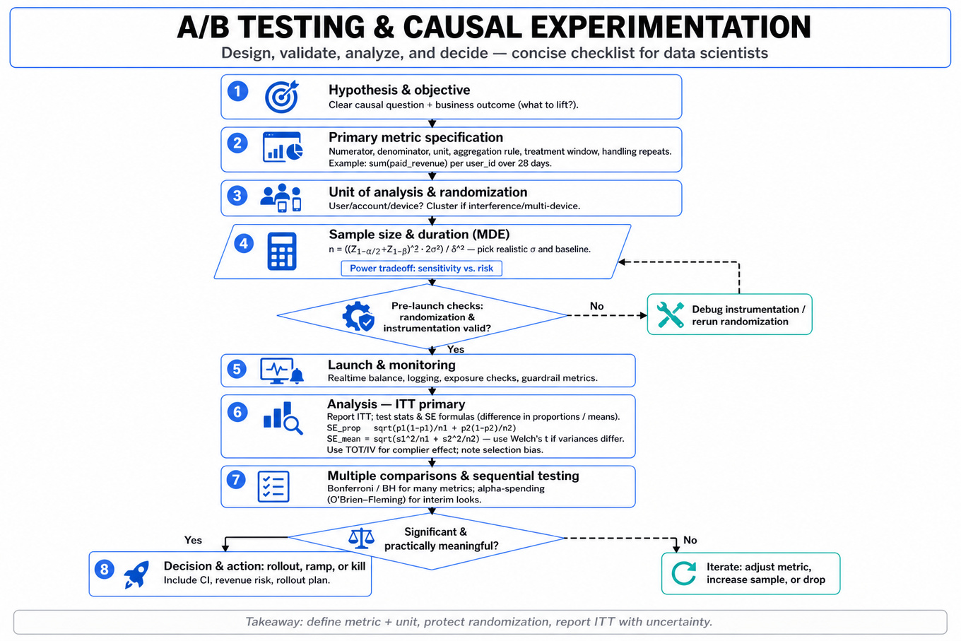
These interviews probe a candidate’s ability to design, analyze, and defend causal experiments end-to-end: picking a precise primary metric, sizing and timing an experiment, choosing randomization and analysis methods that respect the unit-of-analysis, diagnosing instrumentation or randomization failures, and translating statistical lift into product recommendations. Google expects Data Scientists to reason about tradeoffs between sensitivity (power), risk (user and revenue impact), and operational constraints while communicating uncertainty clearly.

Core knowledge

• Unit of analysis: Define the experiment at the correct level (user, account, cookie, device). Mismatch causes biased SEs and misleading p-values; cluster randomization when interference or multi-device users exist.
• Primary metric construction: Precisely specify numerator, denominator, unit, aggregation rule, treatment window, and handling of repeated observations (per-user mean, per-event rate, or sum). Example: primary = sum(paid_revenue) per user_id over 28 days.
• Test statistic & SE formulas: For difference in proportions, use $SE=\sqrt{\frac{p_1(1-p_1)}{n_1}+\frac{p_2(1-p_2)}{n_2}}$; for means, $SE=\sqrt{\frac{s_1^2}{n_1}+\frac{s_2^2}{n_2}}$. Use Welch's t when variances differ.
• Sample size / MDE calc: For two-sided mean test, with equal n: $n=\frac{(Z_{1-\alpha/2}+Z_{1-\beta})^2\cdot 2\sigma^2}{\delta^2}$ where $\delta$ is minimum detectable effect (MDE). Use realistic baseline variance and conversion rates.
• Intent-to-treat (ITT) vs. Treatment-on-treated (TOT): Report ITT as primary; use TOT or instrumental variables to estimate complier effect if noncompliance exists, but note selection bias.
• Covariate adjustment & CUPED: Use pre-period covariates in ANCOVA to reduce variance; CUPED uses a pre-experiment metric to lower $\sigma^2$ and increase power without biasing ITT.
• Multiple comparisons & sequential testing: Control Type I with Bonferroni / BH for many metrics, or use alpha-spending / group-sequential methods (e.g., O’Brien–Fleming) for interim looks; false discovery is common with dashboards.
• Heterogeneous treatment effects: Pre-specify subgroups and interaction tests; beware data-dredging. Use regression with interaction terms for exploratory HTE, and correct for multiplicity when making decisions.
• Duration, ramping, and seasonality: Account for weekdays, marketing events, and user lifecycle. Ensure experiment runs long enough to stabilize metrics (behavioral latency, billing cycles).
• Diagnostics & instrumentation checks: Always run Sample Ratio Mismatch (SRM), unit-consistency tests, pre-period balance, and event-logging completeness. SRM often indicates assignment or logging bugs.
• Non-standard outcomes: For retention or survival outcomes, use Kaplan–Meier and log-rank tests or Cox models for time-to-event; use bootstrap for skewed revenue/LTV.
• Interference & SUTVA violations: If users interact (social features), consider network experiments or cluster/graph-randomization; standard A/B assumptions break otherwise.

Worked example — "Design A/B Test for Subscription Price Increase Effectiveness"

First 30 seconds: clarify the objective (maximize long-run revenue vs. short-term conversion), unit (account or user), and acceptable business constraints (max allowable conversion drop). Pillars of the answer: (1) metric design — primary = 90-day discounted LTV per account_id with secondary metrics conversion_rate and churn; (2) experimental design — randomized rollout at account level, stratify by historical spend or geography; (3) sizing and ramp — compute MDE for revenue per user using baseline mean and variance, plan minimum 8-week run to capture billing cycle; (4) analysis — use ITT for decision-making, regress revenue on treatment with covariate adjustment (ANCOVA), and report bootstrap CI for skewed revenue. Tradeoff to flag: powering for revenue requires large N because variance is high; if business cannot afford long runs, consider powering on conversion (easier) but note mismatch with revenue objective. Close: state guardrails (abort on SRM, large negative churn) and say, "if more time, I'd run a small pilot to validate instrumentation, estimate variance, and consider a price ladder (factorial) to learn elasticity."

A second angle — "Boost Google Workspace Chat Usage with Strategic A/B Testing"

Here the goal is engagement uplift, so metrics and interference look different: primary could be DAU per user or session frequency, and unit is often user_id. Social features create network effects — randomizing at user-level may cause contamination between treated and control (messages cross). You'd consider cluster randomization by team/organization or use exposure modeling. Because engagement changes can be small, use variance reduction (CUPED) and pre-specify subgroup analyses (new users vs. power users). Operationally, real-time metrics and funnel diagnostics matter: if initial increases are from notifications, monitor downstream effects like notification fatigue.

Common pitfalls

Pitfall: Unit-of-analysis mismatch — randomizing on cookie or device while reporting per-user metrics. This underestimates variance and can produce false positives. Always align randomization and analysis unit or use cluster-robust SEs.

Pitfall: Reporting an unanchored metric — saying "lift in conversion = 2%" without stating baseline rate, observation window, or whether it's ITT. Interviewers expect numerator/denominator and CI or p-value.

Pitfall: Ignoring runtime diagnostics and SRM — a statistically significant lift that coincides with a sample-ratio mismatch or logging changes is unreliable. Run SRM, event-completeness, and pre-period balance as part of the analysis pipeline.

Connections

Experimentation work commonly pivots into causal inference on observational data (difference-in-differences, propensity scores) when randomization isn't feasible, or into metric monitoring and anomaly detection to spot experiments that leak. Interviewers may also pivot to ranking/recommender evaluation when experiments affect A/B ranking metrics.

Further reading

• Practical Guide to Controlled Experiments on the Web (Kohavi et al.) — a canonical, practical overview of online A/B testing.
• Evan Miller, A/B Testing: The Complete Guide — hands-on explanations of sample size, sequential testing, and pitfalls.

Practice questions

Focus area — Google-specific addendum for ranking metrics, interleaving, offline-online gaps, and guardrails, aligned with your weak experimentation and metric-design signals.

What's being tested

This topic tests whether you can evaluate search ranking changes with metrics that reflect user utility rather than merely counting clicks. You should be able to distinguish offline relevance evaluation from online experimentation, explain why standard A/B tests can require substantial traffic, and use interleaving to compare rankers efficiently within the same search session. Google cares because small ranking changes affect billions of impressions, and a Data Scientist must separate genuine relevance improvements from position bias, novelty effects, query mix changes, and noisy user behavior.

Core knowledge

• Ranking evaluation starts by defining the unit of analysis: query, query-user session, impression, or task completion. Offline metrics such as NDCG@k, MRR, MAP, and recall measure different objectives; online metrics such as click-through rate, reformulation rate, abandonment, and long-click rate capture realized behavior.

• Discounted cumulative gain values highly relevant documents near the top:
  $DCG@k=\sum_{i=1}^{k}\frac{2^{rel_i}-1}{\log_2(i+1)}$
  Normalize by the ideal ordering to obtain NDCG@k; use graded labels when “excellent” and “acceptable” results should not count equally.

• Interleaving combines results from two rankers into one displayed list, then attributes user interactions to the ranker contributing the clicked result. It controls much of the query and user heterogeneity because both rankers compete within the same impression rather than across separate users.

• Team Draft interleaving alternates turns: each ranker selects its highest-ranked document not already included, with a randomized first picker. It is simple and interpretable, but duplicate results, unequal candidate overlap, and position-dependent click behavior can create attribution bias.

• Balanced Interleaving or probabilistic interleaving samples among valid combined lists so each ranker receives comparable exposure. The design should define how probabilities are computed and use inverse-probability weighting if displayed positions or assignments are not equally likely.

• The primary interleaving outcome is often a win rate or preference statistic:
  $\hat{p}=\frac{\text{wins}_A+\frac{1}{2}\text{ties}}{\text{wins}_A+\text{wins}_B+\text{ties}}$
  Analyze at the query or session level, not as independent clicks, because one session may generate multiple correlated interactions.

• Position bias means users are more likely to click higher-ranked results even when relevance is identical. Interleaving reduces common exposure differences, but it does not eliminate bias; inspect clicks by position, use randomized first selection, and consider click models such as examination models or propensity weighting.

• A click is an imperfect relevance label: attractive titles, navigational intent, brand familiarity, and result snippets affect it. Pair click outcomes with long clicks, rapid backtracks, query reformulations, dwell time, task completion, explicit judgments, or satisfaction surveys, while recognizing that dwell time itself can be confounded by page type.

• Statistical inference must match the randomization unit. Use paired analyses or clustered standard errors by query, user, or session; report confidence intervals and practical effect sizes. A tiny statistically significant preference may not justify latency, infrastructure, or product risk.

• Sample-ratio mismatch and instrumentation checks precede interpretation. Verify traffic assignment, ranker eligibility, logging completeness, duplicate handling, bot filtering, and treatment exposure before trusting a preference estimate. A missing click can look like a ranker loss.

• Query heterogeneity matters: navigational, informational, transactional, head, tail, fresh, multilingual, and mobile queries can respond differently. Pre-specify segments, control multiple comparisons, and report both aggregate and segment-level effects so a gain on head queries does not conceal tail-query harm.

• Offline-online disagreement is expected. Human labels may reward topical relevance while users reward freshness or authority; static test sets miss query drift and feedback loops. Use offline metrics for fast iteration, interleaving for sensitive pairwise comparison, and randomized A/B tests for final product-level impact.

Worked example — “Compare Two Search Rankers Using Interleaving”

A strong candidate would first clarify whether the goal is pairwise relevance comparison, launch approval, or diagnosis, and whether the unit of randomization is query, session, or user. They would state assumptions: both rankers return eligible results for the same query, clicks are logged reliably, and the primary outcome is a pre-specified session-level preference rather than raw click count. The answer would be organized around four pillars: candidate-list construction, an interleaving algorithm, unbiased outcome attribution, and statistical analysis with guardrails. They might choose Team Draft for interpretability, randomize the first picker, and define deterministic duplicate handling before looking at results. They would explicitly flag the tradeoff between simple attribution and exposure bias, noting that probabilistic interleaving may reduce bias but be harder to explain and implement. They would compare win rate, tie rate, clicks per session, reformulations, and latency while checking query-type and device segments. They would validate logging and run an A/A test to detect assignment or attribution problems. If they had more time, they would calibrate the result against judged NDCG@10, investigate disagreement queries, and follow with a properly powered user-level A/B test.

A second angle — “Diagnose a Ranking Metric Mismatch”

Here the same concept is framed around a case where NDCG@10 improves but interleaving preference and long-click rate decline. The candidate should ask whether the gains are concentrated in a narrow query segment, whether labels are stale, and whether the new ranker changes result diversity or freshness. They should inspect position-specific clicks, reformulations, abandonment, and query-level paired outcomes rather than declaring the online metric wrong. A plausible explanation is that the offline labels reward topical relevance while users prefer direct answers or authoritative destinations for current queries. The next step is to identify disagreement cohorts, obtain targeted human judgments, and run a controlled experiment with guardrail metrics.

Common pitfalls

Pitfall: Saying “the ranker with more clicks wins” ignores exposure, duplicate results, position bias, and session correlation. Define attribution before observing outcomes, use the randomization unit for inference, and report uncertainty around a paired preference estimate.

Pitfall: Presenting one aggregate win rate as a launch decision hides important heterogeneity. A stronger answer names the primary metric, guardrails, minimum practical effect, key cohorts, and the conditions under which the decision would change.

Pitfall: Treating interleaving as a replacement for an A/B test overstates what it identifies. Interleaving is excellent for sensitive pairwise ranker comparison, but it does not fully estimate absolute product impact, latency effects, ecosystem effects, or long-term behavior; validate promising results with randomized experimentation.

Connections

An interviewer may pivot to counterfactual evaluation, click models, A/B test power analysis, multiple-hypothesis correction, or human relevance judgments. They may also ask how ranking quality interacts with latency, diversity, freshness, fairness, and personalization.

Further reading

• “Unbiased Learning-to-Rank with Biased Feedback” — Joachims et al. — foundational treatment of position bias and propensity-based correction.

• “Efficient Online Evaluation of Ranking Systems” — Chapelle et al. — practical analysis of interleaving and online ranker comparison.

• “Search Result Diversification” — Santos, Macdonald, and Ounis — useful context for evaluating relevance when multiple intents and result types matter.

Practice questions

Focus area — Analytics is 1/5, and your selected focus includes metric design, segmentation-style reasoning, causal threats, and impact quantification.

What's being tested

Interviewers are probing the candidate's ability to define actionable, measurable user segments, validate their stability and separability over time, and tie segments to causal evaluation (experimentation) and product metrics. Expect questions on cohort construction, metric definitions and guardrails, statistical power and correction for multiple comparisons, and how segmentation drives targeted interventions with clear success criteria.

Core knowledge

• Segment definition: A good segment is defined by reproducible rules (behaviors, device, geography, engagement thresholds) expressible as SQL filters against event tables; prefer deterministic keys (user_id, mail_hash) over heuristics.

• Cohort vs. segment: Cohort analysis groups users by an anchor event/time (e.g., first signup week), while segmentation can be static or rolling; both require clear enrollment and look-back windows.

• Metric taxonomy: Distinguish activation, engagement (e.g., DAU, sessions/day), retention (e.g., 7-day retention), and quality (deliverability, spam rates); each needs an explicit numerator/denominator and handling for event deduplication.

• MoM & percent-change math: Month-over-month percent change = $\frac{V_{t}-V_{t-1}}{V_{t-1}} \times 100\%$ — handle zero/near-zero denominators with smoothing or reporting absolute change.

• Statistical testing basics: For A/B, report point estimate, confidence interval, and p-value; use pooled vs. unpooled tests appropriately and always show direction and magnitude, not just significance.

• Sample size & power: For binary metrics, approximate sample size per group: $n \approx \frac{(Z_{1-\alpha/2}+Z_{1-\beta})^2 (p_1(1-p_1)+p_2(1-p_2))}{(p_1-p_2)^2}$ — explicitly state minimum detectable effect (MDE).

• Multiple comparisons & FDR: When testing many segments, control family-wise error (Bonferroni) or prefer false discovery rate (Benjamini–Hochberg) to maintain interpretability across dozens of cohorts.

• Stability & separability checks: Use time-series correlation, silhouette scores for feature separability, and validate segment sizes over rolling windows to detect population drift.

• Causal inference alternatives: For non-randomized targeting, rely on propensity score matching, difference-in-differences, or instrumental variables; always assess confounding and overlap.

• Metric decomposition & attribution: Decompose overall KPI moves into segment-level contributions: $\Delta KPI = \sum_s w_s \Delta KPI_s + \sum_s \Delta w_s KPI_{s,baseline}$ to understand whether change comes from behavior within segments or composition shifts.

• Privacy & safety: Use differential privacy, aggregate reporting thresholds, or only publish segments above minimum N to avoid deanonymization; treat mailbox content as off-limits — rely on metadata.

• Practical tools: Query/analysis commonly done in BigQuery/Postgres; visualization and dashboards in Looker; for experiments, reference platforms like Experimentation frameworks that provide exposure logs and assignment hashes.

Worked example — Define and apply Gmail user segments

Clarify first: ask which signals are available (events, timestamps, device, inbox actions), the business goal (growth, retention, spam reduction), and privacy constraints (no message content). Frame the analysis into three pillars: (1) Define segments by behavior (e.g., "power users" = >20 sends/week and uses >2 devices), (2) Validate by checking size, stability over 8 weeks, and separability (time-series and feature distributions), (3) Action & evaluation design targeted interventions with metrics and guardrails. A strong candidate sketches SQL-derived cohort queries, lists primary and guardrail metrics (e.g., primary: weekly active senders; guardrail: spam-rate and latency), and computes sample-size/MDE per segment to decide whether to run per-segment A/B tests or pooled experiments with interaction analysis. Explicit tradeoff: smaller, high-value segments enable personalized impact but reduce power and increase multiple-testing burden; consider hierarchical testing or pooled tests with pre-specified segment interactions. Close by saying: if given more time, I'd prototype the segment queries, run an initial stability dashboard, and simulate power using historical variance to decide test allocation.

A second angle — Calculate Top Countries' Gmail Usage and MoM Change

This task focuses on time-based aggregation and window functions rather than segmentation. Start by clarifying the event grain (per-message, per-session), the country attribution logic (IP, account profile), and timezone normalization. Main pillars: (1) Aggregate counts per country/month in BigQuery, (2) rank countries using ROW_NUMBER() OVER (PARTITION BY month ORDER BY volume DESC), (3) compute MoM with LAG() and handle zero denominators and late-arriving events. A key tradeoff is whether to compute on raw event streams (more precise but heavier) or daily rollups (faster but may hide freshness issues). If asked to extend, propose normalizing by active users per country to report per-user usage instead of raw volume to avoid conflating population size with engagement.

Common pitfalls

Pitfall: Defining segments by noisy or transient signals.

Many candidates craft segments from one-off events (e.g., "opened promo last week") that aren't stable; better to require repeat behavior or use rolling windows to ensure stability and assign membership consistently.

Pitfall: Ignoring multiple-testing when reporting per-segment significance.

Reporting many per-segment p-values without FDR control leads to false positives; explicitly plan correction strategy (hierarchical testing, BH procedure) and pre-specify primary segments.

Pitfall: Focusing only on statistical significance, not practical impact.

Saying a change is "significant" without showing absolute lift, baseline rate, or potential negative guardrails (e.g., higher spam complaints) fails to inform product decisions; always surface magnitude and risk.

Connections

Interviewers may pivot to experiment design at scale (sequential testing, stopping rules) or personalization ranking (offline metrics like NDCG, online CTR uplift by segment). They may also ask about privacy-preserving analytics (aggregation thresholds, noise addition) when segments get small.

Practice questions

Focus area — You flagged metric design, causal diagnostics, and experimentation gaps; YouTube questions combine those with latency, engagement, and guardrail trade-offs.

What's being tested

These cases test whether you can turn ambiguous product questions into measurable outcomes, credible comparisons, and actionable diagnoses. You must connect metric definitions, randomization, causal inference, segmentation, and model adjustment rather than treating engagement as a single number. Google cares because small measurement errors can drive decisions affecting ranking, advertising quality, creator incentives, and billions of viewing sessions.

Core knowledge

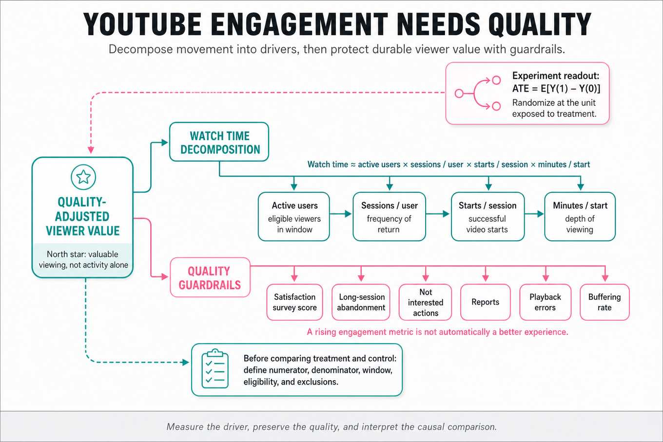
• Metric trees decompose DAU or watch time into interpretable factors: active users × sessions per user × starts per session × minutes per start. Define numerator, denominator, window, eligibility, and exclusions before analyzing movement.

• North-star metrics should represent durable user value, not merely activity. Pair watch time or successful video starts with quality guardrails such as satisfaction surveys, long-session abandonment, “not interested” actions, reports, errors, and buffering.

• Randomized controlled experiments estimate an average treatment effect: $\text{ATE}=E[Y(1)-Y(0)]$. Randomize at the unit exposed to treatment—viewer, session, device, or region—and choose the unit to limit contamination and interference.

• Interference violates the usual stable-unit assumption when one viewer’s treatment changes another viewer’s outcomes, such as shared recommendations or social viewing. Consider user-level assignment, cluster randomization, geo experiments, or exposure-based analyses, while acknowledging reduced power.

• Power analysis depends on baseline variance, minimum detectable effect, significance level, and traffic allocation. For a proportion, approximate standard error is $\sqrt{p(1-p)/n}$; use historical variance and account for clustering, repeated users, and multiple primary metrics.

• Latency experiments should distinguish client-perceived video-start latency from backend request latency. Analyze treatment effect on starts, watch time, retention, and abandonment, while guarding against buffering, playback errors, startup quality, and users receiving fewer starts because they quit earlier.

• Mixed-effects regression separates systematic item differences from reviewer severity: $y_{ij}=\beta_0+\alpha_i+u_j+\epsilon_{ij}$, where $\alpha_i$ is an ad fixed effect and $u_j\sim N(0,\sigma_u^2)$ is a reviewer random effect. Adjusted ad scores remove estimated reviewer composition bias.

• Shrinkage in hierarchical models pulls noisy reviewer or ad estimates toward the population mean, especially with few observations. Validate with held-out reviewers, residual checks, calibration, and sensitivity to random-effect distributions; do not present adjusted scores as causal truth automatically.

• Ordinal outcomes such as one-to-five ratings may violate linear-regression assumptions. Compare linear mixed models with cumulative-logit mixed models, inspect whether conclusions and rankings are stable, and communicate whether the score is predictive, descriptive, or decision-oriented.

• Segmentation and cohorts localize changes by platform, country, app version, acquisition channel, new versus returning users, device class, and exposure to launches. Pre-specify meaningful segments, control false discoveries, and distinguish composition shifts from within-segment behavior changes.

• Instrumentation validation precedes causal storytelling: reconcile client and server counts, inspect event coverage, compare stable dashboards, and check timestamp or definition changes. Upstream logs and experiment-exposure tables are evidence sources to query, not pipeline components to redesign.

Worked example

For “Design tests to measure latency impact,” I would first clarify which latency—tap-to-first-frame, time to playable, or request completion—is changing, and whether the goal is engagement, satisfaction, or both. I would state that the primary outcome is a pre-specified metric such as successful starts per eligible session or watch time per user, with startup abandonment and buffering as guardrails. My answer would have four pillars: treatment assignment, power and analysis, quality diagnostics, and heterogeneity or long-term effects. I would randomize at the viewer level if treatment can persist across sessions, define eligibility before exposure, and use intention-to-treat as the primary estimate. I would explicitly flag the tradeoff between session-level randomization, which may increase contamination, and user-level randomization, which improves treatment consistency but requires more users and can create persistent user experience differences. I would verify balance, estimate confidence intervals, inspect quantiles and early exits, and check that reduced startup latency is not purchased through worse playback stability. I would segment by device, network type, geography, and new versus returning viewers, but treat those results as exploratory unless powered or corrected. If I had more time, I would add a longer holdout to test retention and examine whether repeated exposure changes behavior.

A second angle

For “Diagnose YouTube Usage Decline: Key Metrics and Segmentation,” the same discipline applies without a randomized treatment: first establish whether the decline is real, then decompose it into population, frequency, and per-session components. The main challenge is separating instrumentation or denominator changes from genuine behavior, so compare multiple independent definitions and unaffected reference metrics. Segmentation becomes a hypothesis-generation tool rather than proof of causality; a platform-specific decline may reflect rollout exposure, user composition, or an external outage. The strongest close proposes a targeted experiment or quasi-experimental comparison to validate the suspected cause.

Common pitfalls

Pitfall: Treating watch time as unambiguously positive. More minutes can result from slower playback, compulsive low-quality consumption, or fewer alternative activities; pair it with satisfaction and quality guardrails and explain the decision metric.

Pitfall: Saying “randomize users and compare means” without defining exposure, interference, power, or the primary metric. A stronger answer names the assignment unit, estimand, analysis population, confidence interval, and failure modes that could invalidate interpretation.

Pitfall: Overclaiming from a mixed-effects model or a descriptive segment. Reviewer random effects can adjust composition bias, but they do not prove rating validity; similarly, a declining Android cohort does not establish that an Android change caused the overall decline.

Connections

An interviewer may pivot to sequential testing, multiple-hypothesis correction, difference-in-differences, survival analysis, or ranking evaluation. Be ready to connect product metrics to offline relevance measures such as NDCG while explaining why online user outcomes remain the decision criterion.

Further reading

• Trustworthy Online Controlled Experiments — Ron Kohavi, Diane Tang, and Ya Xu’s practical treatment of experimentation, guardrails, power, and novelty effects.

• The Design and Analysis of Split-Plot Experiments — useful grounding for clustered assignment and dependence structures.

• Gelman and Hill, Data Analysis Using Regression and Multilevel/Hierarchical Models — a rigorous reference for partial pooling and mixed-effects modeling.

Practice questions

Statistics & Math

Focus area — You marked Simpson’s paradox and ratio denominator effects shaky, and selected causal inference, sampling bias, and weighted estimation.

What's being tested

These questions test whether you can recognize when an aggregate comparison reverses or obscures the pattern seen within meaningful subgroups. The interviewer is probing confounding, composition effects, weighted averages, and the distinction between descriptive association and causal effect. For a Data Scientist at Google, this matters because product metrics, experiment results, ranking quality, and user behavior are routinely aggregated across countries, devices, user cohorts, traffic sources, or query difficulty levels.

Core knowledge

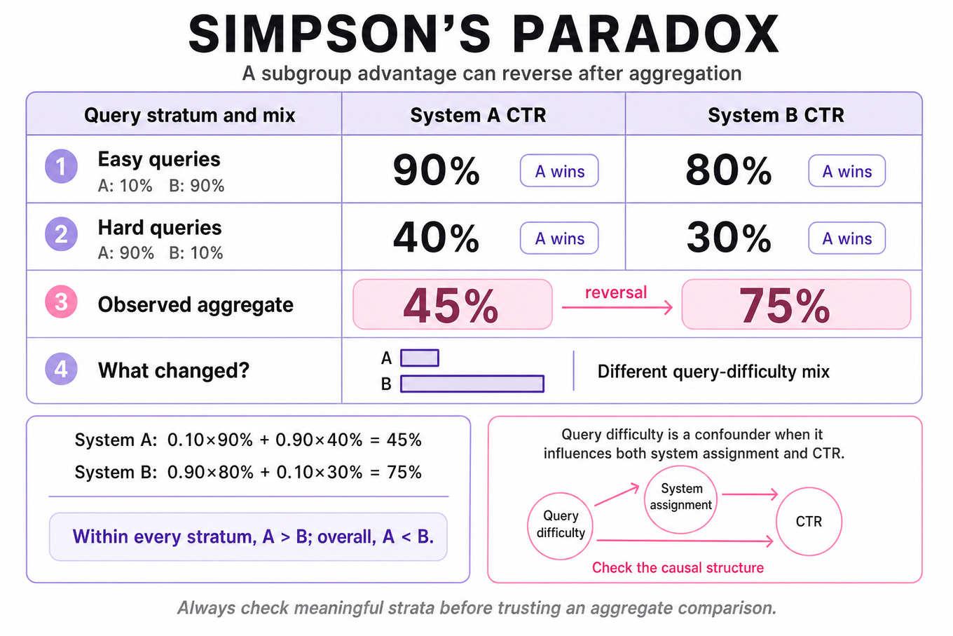
• Simpson’s paradox occurs when the direction or interpretation of an association changes after data is partitioned by a third variable. A treatment can outperform control in every subgroup yet appear worse overall because treatment and control have different subgroup proportions.

• Aggregates are weighted averages, not simple averages. For subgroup rates $r_i$ with weights $w_i$, the overall rate is $\sum_i w_i r_i$, where $\sum_i w_i=1$. A reversal is possible when the treatment groups have substantially different weights across strata.

• A confounder influences both the exposure and outcome, creating a non-causal association. For example, query difficulty may affect both ranking-system assignment and click-through rate; comparing systems without controlling for difficulty can mislead.

• Distinguish confounding from mediation and collider bias. Adjusting for a mediator can remove part of the effect you want to estimate, while conditioning on a collider—affected by both exposure and outcome—can create a spurious association.

• Start with a causal graph or explicit estimand: for example, “the average treatment effect of ranking system A versus B on qualified clicks among eligible searches.” The correct adjustment set depends on that causal question, not merely on correlated variables.

• Stratification estimates subgroup-specific effects, such as $\hat{\tau}_s=\bar{Y}_{T,s}-\bar{Y}_{C,s}$. To estimate a population effect, standardize using a common target distribution: $\hat{\tau}_{pop}=\sum_s p_s(\bar{Y}_{T,s}-\bar{Y}_{C,s})$.

• In randomized experiments, treatment is independent of pre-treatment covariates in expectation, so randomization protects against confounding. However, chance imbalance, noncompliance, differential missingness, or post-treatment conditioning can still distort practical analysis.

• For a ratio metric such as CTR = clicks / impressions, inspect numerator and denominator separately, then segment by high-impact dimensions. A change may reflect traffic mix, exposure volume, or denominator composition rather than a genuine per-impression behavioral change.

• Standardization and regression adjustment answer different operational needs. Standardization is transparent for a few important strata; regression, inverse-probability weighting, or doubly robust estimators scale better but require modeling assumptions and overlap.

• Check overlap, also called positivity: every relevant subgroup should have meaningful observations under both conditions. If one ranking system serves almost exclusively easy queries, within-stratum comparisons may be noisy or impossible.

• Statistical uncertainty matters after stratification. Small subgroups can show extreme rates by chance, so report confidence intervals or posterior intervals, account for multiple comparisons when scanning many segments, and avoid selecting only “significant” reversals.

• Not every reversal is paradoxical or erroneous. It may reflect a real population shift, a policy change, a meaningful target-population difference, or a valid difference between an overall estimand and a conditional estimand. Explain which population the metric is intended to represent.

Worked example

For “Explain and resolve Simpson’s paradox,” I would first clarify whether the interviewer wants a descriptive explanation, a causal treatment effect, or a product-metric diagnosis, and I would ask what variable defines the relevant subgroups. I would state the core pattern: an aggregate comparison can reverse because subgroup rates are weighted by different population mixes. I would organize the answer around four pillars: show subgroup tables, compute the aggregate weighted rates, identify the confounding or composition variable, and choose an estimand-appropriate resolution. For instance, if a new search system wins for both easy and hard queries but receives mostly hard-query traffic, I would not call the aggregate result a simple system failure without examining query mix. I would compare within-query-difficulty effects and then standardize both systems to the same difficulty distribution. The explicit tradeoff is that stratification improves interpretability but can increase variance or fail when some strata lack overlap; regression or hierarchical modeling may stabilize estimates while adding assumptions. I would close by saying that I would also check randomization integrity, missing outcomes, metric definitions, and confidence intervals before recommending a product decision.

A second angle

For “How do you diagnose a ratio metric change,” the same idea appears through numerator-denominator composition rather than a treatment table alone. I would decompose the ratio, compare segment-level rates and traffic weights, and test whether the overall movement is driven by a shift toward segments with systematically higher or lower baselines. The key framing is diagnostic: first establish whether instrumentation or denominator changes explain the movement, then determine whether the within-segment behavior changed. I would also distinguish an intended population change from a misleading aggregate artifact. A useful next step is to report both the observed metric and a composition-adjusted metric using a fixed reference distribution.

Common pitfalls

Pitfall: Saying “always adjust for the third variable” is analytically wrong. Adjustment is appropriate for a pre-treatment confounder, but conditioning on a collider or mediator can bias the estimand; first define the causal question and draw the likely relationships.

A tempting answer gives only a toy reversal table and declares the paradox “resolved” by averaging subgroup percentages. That ignores unequal subgroup sizes: show the weights, compute aggregate rates, and explain whether the desired quantity is the observed population effect or a standardized comparison.

Some candidates attribute every reversal to bad data or randomization failure. A stronger answer acknowledges genuine population shifts, overlap limitations, uncertainty, and multiple possible estimands, then proposes concrete checks such as segment-level confidence intervals and a pre-specified reference distribution.

Connections

An interviewer may pivot to causal diagrams, randomized experiments, inverse-probability weighting, or ratio-metric variance. Related topics include heterogeneous treatment effects, multiple-hypothesis testing, missing-data bias, and transportability from an experiment population to the product population.

Further reading

• Causality — Judea Pearl — Formal treatment of confounding, adjustment, causal graphs, and Simpson’s paradox.

• Causal Inference: What If — Hernán and Robins — Free, rigorous reference for standardization, inverse-probability weighting, and causal estimands.

• The Book of Why — Judea Pearl and Dana Mackenzie — Accessible intuition for causal reasoning and why association alone is insufficient.

Practice questions

Focus area — You selected resampling and Monte Carlo, and several inference and sampling concepts are shaky or new.

What's being tested

These problems test whether you can define a truncated normal distribution, normalize its density correctly, and generate samples from it without introducing bias. The interviewer is probing your command of inverse-CDF sampling, rejection sampling, tail behavior, and the numerical tradeoffs among competing Monte Carlo methods. For a Data Scientist, this matters when modeling censored or constrained measurements, simulating counterfactuals, estimating uncertainty, or validating an estimator whose inputs are observed only within a range.

Core knowledge

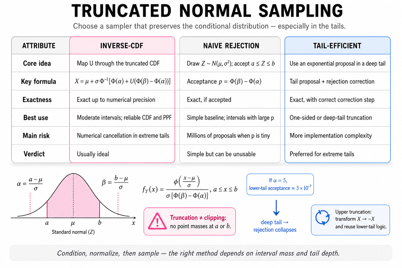
• A truncated normal is a normal random variable conditioned to lie in $[a,b]$: $X\sim N(\mu,\sigma^2)\mid a\le X\le b$. It is not the same as clipping values to the boundaries, which creates point masses at $a$ and $b$.

• Let $\alpha=(a-\mu)/\sigma$ and $\beta=(b-\mu)/\sigma$. The normalized density is $f_T(x)=\frac{\phi((x-\mu)/\sigma)}{\sigma[\Phi(\beta)-\Phi(\alpha)]},\qquad a\le x\le b,$ where $\phi$ and $\Phi$ are the standard normal PDF and CDF.

• Its CDF is

  {\Phi(\beta)-\Phi(\alpha)}.$$ This formula is the key to deriving both quantiles and **inverse-CDF sampling**; omitting the denominator incorrectly leaves the distribution unnormalized.

• Inverse-CDF sampling draws $U\sim\mathrm{Uniform}(0,1)$ and returns $X=\mu+\sigma\Phi^{-1}\left[\Phi(\alpha)+U\{\Phi(\beta)-\Phi(\alpha)\}\right].$ It is exact up to numerical precision and usually ideal for moderate intervals when reliable normal_cdf and normal_ppf implementations exist.

• Rejection sampling proposes $Z\sim N(\mu,\sigma^2)$ repeatedly and accepts it when $a\le Z\le b$. It is simple and exact, but its expected number of proposals is $1/p$, where $p=\Phi(\beta)-\Phi(\alpha)$. It becomes unusable when $p$ is extremely small.

• For one-sided lower truncation $X\ge a$, naive rejection has acceptance probability $1-\Phi(\alpha)$. If $\alpha=5$, this is roughly $3\times10^{-7}$, so millions of proposals may be needed per accepted draw.

Tip: Use a tail-efficient sampler, such as exponential rejection methods, for deep tails.

• For an upper truncation, transform signs: if $X\sim N(\mu,\sigma^2)$ conditioned on $X\le b$, then $-X$ is lower-truncated at $-\!b$ with mean $-\mu$. This reduces implementation complexity and helps reuse a well-tested lower-tail routine.

• Inverse-CDF calculations can lose precision when $\Phi(\alpha)$ is extremely close to $1$ or when $\Phi(\beta)-\Phi(\alpha)$ suffers catastrophic cancellation. Use stable survival-function APIs such as logsf, log-CDF arithmetic, or specialized truncated-normal libraries for extreme tails.

• The conditional mean is

  {\Phi(\beta)-\Phi(\alpha)}.$$ The conditional variance is $$\sigma^2\left[1+\frac{\alpha\phi(\alpha)-\beta\phi(\beta)} {\Phi(\beta)-\Phi(\alpha)} -\left(\frac{\phi(\alpha)-\phi(\beta)} {\Phi(\beta)-\Phi(\alpha)}\right)^2\right].$$ These are useful checks for simulations.

• Monte Carlo error decreases as $O(1/\sqrt n)$, not $O(1/n)$. To halve the standard error, you need approximately four times as many draws. Use independent random seeds, report uncertainty, and verify empirical moments or quantiles against theoretical values.

• Distinguish truncation from censoring and selection bias. Truncation removes observations outside a range; censoring records them only as “below” or “above” a threshold. Treating a censored sample as an ordinary truncated sample can bias parameter estimates and downstream experiment metrics.

Worked example: Define and sample a truncated normal

A strong candidate would first ask whether the interval is finite or one-sided, whether the goal is a mathematical derivation or production-quality sampling, and whether extreme-tail numerical stability matters. I would state that $X\sim N(\mu,\sigma^2)$ is conditioned on $a\le X\le b$, then organize the answer around the normalized PDF, the CDF, an exact sampling algorithm, and validation checks. I would derive the acceptance probability $p=\Phi(\beta)-\Phi(\alpha)$ before choosing between inverse-CDF and rejection sampling. The default implementation would use inverse-CDF sampling because it gives one accepted draw per uniform variate and avoids rejection inefficiency. I would explicitly flag the tradeoff that inverse-CDF is computationally predictable but can be numerically delicate in extreme tails, whereas rejection sampling is easier to explain but may be catastrophically slow there. I would validate simulated mean, variance, interval membership, and a histogram or probability integral transform against the theoretical distribution. I would also clarify whether parameters are known or estimated, because fitting a truncated likelihood requires including the same normalization constant. If I had more time, I would benchmark a tail sampler and test behavior across very narrow intervals and large standardized cutoffs.

A second angle: Generate Samples from Truncated Normal Distribution

For lower-tail truncation, the central issue shifts from deriving the bounded-interval formulas to algorithmic efficiency when $X\ge a$ and $a$ is many standard deviations above $\mu$. Inverse-CDF remains conceptually clean, but evaluating $1-\Phi(\alpha)$ directly may underflow or lose precision. A strong answer compares naive rejection with exponential-envelope or specialized normal-tail samplers and quantifies acceptance rather than merely naming methods. The practical choice depends on the tail threshold, sample volume, and whether the environment provides stable logsf and ppf functions.

Common pitfalls

Pitfall: Saying “sample a normal and clip values outside the interval” is wrong because clipping creates boundary point masses and does not produce the conditional distribution. State clearly that rejected values must be resampled, or use the inverse conditional CDF.

A tempting answer gives the correct PDF but forgets the normalization term $\Phi(\beta)-\Phi(\alpha)$. That density integrates to the probability of landing in the interval, not to one; explicitly checking the integral and conditional CDF prevents this analytical mistake.

Another weak response lists inverse-CDF and rejection sampling without discussing numerical stability or acceptance rate. A better Data Scientist answer quantifies $1/p$, identifies extreme-tail failure modes, and explains how empirical moments or quantiles would validate the implementation.

Connections

An interviewer may pivot to maximum likelihood under truncation, censored-data models such as Tobit regression, or importance sampling for rare events. They may also connect this to confidence intervals, Bayesian posterior sampling, variance reduction, and the distinction between selection effects and genuine population differences.

Further reading

• Robert, “Simulation of truncated normal variables” — classic methods for efficient simulation, especially in tail regions.

• Robert and Casella, Monte Carlo Statistical Methods — rigorous treatment of rejection sampling, importance sampling, and Monte Carlo error.

• Nadarajah, “Some truncated distributions” — broader formulas and properties for truncated distributions.

Practice questions

Focus area — You selected sampling bias and weighted estimation; Google DS interviews often require privacy-safe measurement under biased or incomplete samples.

What's being tested

This topic tests whether you can measure behavior when user-level data is incomplete, sampled, aggregated, or intentionally protected by privacy controls. You should connect privacy guarantees to estimand definition, sampling bias, weighting, uncertainty, and decision quality rather than treating privacy as a purely engineering constraint. Google cares because products and ads require reliable measurement across large populations while limiting exposure of sensitive individual information. The interviewer is probing whether you can explain what remains identifiable, quantify bias and variance, and recommend a method whose privacy–utility tradeoff matches the decision.

Core knowledge

• An estimand is the precise quantity being measured: for example, the population conversion rate, incremental conversions caused by an ad, or average treatment effect. Define the target population, time window, treatment, outcome, and unit before choosing a privacy-safe estimator.

• Inverse probability weighting (IPW) corrects unequal observation or treatment probabilities. If unit $i$ is observed with probability $\pi_i$, the Horvitz–Thompson estimator is $\hat{T}_{HT}=\sum_i R_i y_i/\pi_i$; unstable small $\pi_i$ values require trimming, stabilized weights, or a redesign.

• A Hájek estimator normalizes weighted totals: $\hat{\mu}_{H}=\frac{\sum_i R_iw_i y_i}{\sum_i R_iw_i}$. It is often less variable than Horvitz–Thompson for means, though normalization can introduce small finite-sample bias and must be included in inference.

• Post-stratification partitions users into cells such as geography, device, age band, or activity level, then weights each cell to known population totals. It reduces selection bias when outcomes are conditionally homogeneous, but sparse or sensitive cells may need merging or suppression.

• Calibration weighting chooses weights satisfying constraints such as $\sum_i w_i x_i = X_{\text{population}}$. Raking is practical for several margins, while entropy balancing or generalized regression can match richer moments; monitor extreme weights and nonconvergence.

• Effective sample size (ESS) reveals variance inflation from weights: $ESS=(\sum_i w_i)^2/\sum_i w_i^2$. A nominal sample of millions can have an ESS of only thousands when a few users dominate, so report both weighted point estimates and ESS.

• Differential privacy (DP) bounds the effect of any one person on released statistics. A mechanism satisfies $(\varepsilon,\delta)$-DP when neighboring datasets have output probabilities differing by at most $e^\varepsilon$, plus $\delta$ failure probability; smaller $\varepsilon$ generally means stronger privacy and more noise.

• For a count with sensitivity $1$, the Laplace mechanism adds noise proportional to $1/\varepsilon$; for bounded sums, sensitivity depends on the outcome range. Clipping contributions before noise addition is essential, but clipping creates bias that should be measured on realistic data.

• Composition consumes a privacy budget across repeated releases. Basic composition adds $\varepsilon$ values, while advanced composition or a privacy accountant can provide tighter bounds; repeated dashboards, slices, and experiments can consume substantially more budget than one headline metric.

• Thresholding and aggregation reduce disclosure risk but are not equivalent to DP. A minimum cohort size, suppression rule, or k-anonymity policy can still leak information through differencing or auxiliary data; assess neighboring releases and correlated metrics.

• Randomized response, local DP, and secure aggregation differ in where protection occurs. Local DP protects before collection but usually has worse utility; central DP gives stronger aggregate accuracy when a trusted curator can add noise; secure aggregation hides individual reports while enabling aggregate computation.

• Privacy-safe causal measurement needs both protected outcomes and valid counterfactuals. In an experiment, estimate an intention-to-treat effect first, preserve randomization, and apply privacy noise or weighting to treatment and control consistently; otherwise, differential noise can create artificial lift.

• For weighted estimates, uncertainty must include sampling and weighting variance, plus privacy noise. A useful approximation is $\operatorname{Var}(\hat{\theta}_{released})\approx\operatorname{Var}(\hat{\theta}_{sampling})+\operatorname{Var}(\eta_{privacy})$, with covariance terms considered when noise or weights are data-dependent.

• Small-cell risk is both a privacy and statistical problem. Suppressing a tiny cohort protects users but can change the estimand; replacing it with a broader cohort, hierarchical shrinkage, or a predeclared “not reported” category is preferable to silently dropping it.

• Validate with sensitivity analysis: compare unweighted, weighted, trimmed-weight, and privacy-noised results; vary clipping thresholds and privacy budgets; and report whether the product decision changes. Privacy protection should be evaluated alongside bias, interval width, subgroup coverage, and reproducibility.

Worked example

Representative question: “How would you estimate campaign conversions when user-level identifiers cannot be shared?”
I would first clarify the estimand—incremental conversions in the target population over a defined window—and ask whether randomized treatment assignment, aggregate cell counts, and population calibration totals are available. I would organize the answer around four pillars: preserve the experimental contrast, correct any sampling or exposure imbalance, apply a formally specified privacy mechanism, and quantify uncertainty and decision sensitivity. If treatment and control aggregates are available by non-sensitive strata, I would compute a weighted difference in means or rates, using stabilized weights and merging sparse cells before release. I would explicitly flag the tradeoff between finer segmentation, which improves bias correction, and larger privacy loss and variance from many released cells. I would add calibrated DP noise to bounded aggregates, track the total privacy budget across repeated queries, and report ESS, confidence intervals, and noise-induced uncertainty. I would close by saying that, with more time, I would run placebo and pre-period balance checks, compare several clipping thresholds, and test whether the launch decision is robust to plausible privacy budgets.

A second angle

Representative question: “How would you report a product metric for a rare user segment without exposing individuals?”
Here the primary challenge is not causal attribution but stable population estimation under small-cell risk. I would define whether the goal is a descriptive rate or a population-representative rate, then consider post-stratification, cell merging, shrinkage, suppression, and DP noise. A broad, predeclared segment may be more useful than a highly granular metric whose ESS is low and whose privacy noise dominates. I would communicate an interval or “insufficient evidence” result rather than presenting a noisy point estimate as precise.

Common pitfalls

Pitfall: Treating a weighted average as automatically unbiased. Weights correct only the selection mechanism they model; unmeasured differences, positivity violations, and extreme weights can leave substantial bias.

Pitfall: Saying “aggregate data is private.” Aggregates can leak through differencing, repeated queries, rare cohorts, or auxiliary information; explain the threat model and use DP, secure aggregation, suppression, or a combination appropriate to it.

Pitfall: Reporting only the privacy parameter. A strong answer also discusses clipping bias, sampling variance, ESS, composition across releases, subgroup utility, and whether the resulting uncertainty changes the product decision.

Connections

The interviewer may pivot to causal inference, randomized experiments, missing-data mechanisms, survey sampling, or differentially private hypothesis testing. Be ready to distinguish measurement error from selection bias and privacy noise from ordinary sampling noise.

Further reading

• “Calibrating Noise to Variance in Privacy-Preserving Data Analysis” — practical treatment of privacy noise and statistical accuracy.

• “The Algorithmic Foundations of Differential Privacy” — foundational definitions, mechanisms, and composition.

• “Survey Sampling” by Leslie Kish — classic grounding in weighting, stratification, and variance.

Practice questions

Focus area — You selected Poisson and count models; event-rate reasoning is useful for searches, clicks, errors, notifications, and reliability incidents.

What's being tested

The interviewer is testing whether you can choose, fit, interpret, and critique count-data models when Google measures events such as searches, clicks, errors, conversions, or notifications. You should distinguish a Poisson rate assumption from alternatives such as negative binomial regression, zero-inflated models, and survival or time-series approaches. Google cares because product decisions often depend on rare-event rates, exposure-adjusted comparisons, and reliable uncertainty estimates—not merely raw event totals. The key is to connect modeling assumptions to metric definition, experimental design, diagnosis, and business interpretation.

Core knowledge

• Poisson distribution models a nonnegative integer count $Y$ over a fixed exposure interval:
  $P(Y=y)=\frac{e^{-\lambda}\lambda^y}{y!}, \qquad E[Y]=Var(Y)=\lambda.$
  The equal-mean-and-variance condition is a useful baseline assumption, not a law of user behavior.

• For event rates, model exposure explicitly: $Y_i\sim\text{Poisson}(e_i\lambda_i)$, where $e_i$ may be user-days, queries, impressions, or device-hours. In a generalized linear model, include $\log(e_i)$ as an offset:
  $\log E[Y_i]=\log(e_i)+\beta_0+\beta^\top x_i.$

• A Poisson regression uses a log link, $\log\mu_i=\beta_0+\beta^\top x_i+\log(e_i)$. A one-unit increase in $x_j$ multiplies the expected rate by $e^{\beta_j}$; report the incidence-rate ratio $e^{\beta_j}$ and its confidence interval.

• Overdispersion occurs when $Var(Y)\gg E[Y]$, commonly because users have heterogeneous propensities, events cluster in sessions, or observations are correlated. A negative binomial model adds latent heterogeneity and typically estimates $Var(Y)=\mu+\alpha\mu^2$.

• Underdispersion is less common but matters when events are constrained or unusually regular. Do not automatically use a negative binomial model simply because counts are involved; inspect the empirical mean–variance relationship and residual diagnostics.

• Exposure and denominator choice define the metric. “Clicks per user,” “clicks per query,” and “clicks per active day” answer different questions. Changing the denominator can change treatment conclusions, especially when treatment affects the number of opportunities.

• Rate ratios are often more interpretable than count differences. If treatment has estimated coefficient $\hat\beta$, the relative lift is $e^{\hat\beta}-1$. For small effects, $\hat\beta$ approximately equals relative lift, but report the transformed value for stakeholder clarity.

• Confidence intervals for a rate should account for the observation process. For a simple Poisson count $Y$ over exposure $E$, $\hat\lambda=Y/E$; exact intervals can use the chi-square distribution, while regression intervals usually come from the coefficient’s standard error or bootstrap.

• Zero inflation means there are more zeros than the chosen count model expects, often because some users cannot or do not participate in the event-generating process. A hurdle model separates “any event” from “how many conditional on participation”; zero-inflated models represent structural and sampling zeros through separate components.

• Repeated observations from the same user violate independence. Use cluster-robust standard errors, generalized estimating equations, random effects, or aggregate to an analysis unit consistent with randomization. In an A/B test, randomization unit and inference unit must be aligned.

• For experiments, prefer an intention-to-treat comparison and pre-specify the exposure denominator, analysis window, guardrails, and handling of users with zero exposure. Avoid conditioning on post-treatment activity unless you can justify the causal estimand.

• For rare events, normal approximations can be poor when counts are small. Aggregate over a meaningful period, use exact or likelihood-based intervals, and distinguish “zero observed events” from “zero true risk”; the former still has an upper confidence bound.

• Model checking should include residuals, observed-versus-predicted counts, dispersion, calibration across exposure bins, and sensitivity to user/session aggregation. A good fit does not prove causality: treatment assignment, confounding, selection, and logging validity remain separate questions.

Worked example

No specific interview title was supplied, so use the representative prompt: “Estimate the rate of search-result clicks per query and compare it across two product variants.” In the first 30 seconds, clarify whether randomization is by user or query, whether every query is eligible for a click, the experiment duration, and whether the target is clicks per query or probability of at least one click. State that the primary estimand is an intention-to-treat rate ratio, with query count as exposure and user-level clustering if users generate repeated queries. Organize the answer around four pillars: metric and exposure definition, Poisson or negative binomial model, uncertainty and experiment validity, and diagnostics or sensitivity analyses. A basic model is $Y_i\sim\text{Poisson}(e_i\lambda_i)$ with treatment indicator in the log-rate equation; the treatment coefficient becomes an incidence-rate ratio. The explicit tradeoff is whether to analyze query-level counts, which is simple but may understate uncertainty from repeated users, or use user-level aggregation, which better respects clustering but can reduce power and change the estimand. I would inspect overdispersion, treatment balance, zero-click behavior, and heterogeneous effects by query type or device. If I had more time, I would compare the count-rate result with a binary click-through analysis and test whether treatment changes the number of eligible queries itself.

A second angle

A different representative prompt is “Model daily notification failures across devices and identify whether a release increased the failure rate.” Here the main challenge is changing exposure: device-days or notification attempts may be more appropriate than raw failures, and devices may have very different baseline risk. A negative binomial or mixed-effects model may be preferable if device-level heterogeneity creates overdispersion. The release effect should be separated from calendar seasonality, traffic composition, and device mix, with confidence intervals clustered at an appropriate unit. If failures are extremely rare, exact rate intervals and aggregation over time may be more defensible than a highly parameterized model.

Common pitfalls

Pitfall: Saying “the Poisson model is appropriate because the outcome is a count” ignores exposure, overdispersion, dependence, and excess zeros. A stronger answer checks the mean–variance relationship, includes an offset, and explains when negative binomial or hurdle models are needed.

Pitfall: Reporting “the coefficient is 0.08” is difficult for a product audience to interpret. Translate it into an incidence-rate ratio: $e^{0.08}-1\approx8.3\%$ relative lift, then state the confidence interval, practical impact, and denominator.

Pitfall: Treating a statistically significant rate increase as automatically causal or desirable misses experiment validity and product tradeoffs. Discuss randomization, guardrail metrics, heterogeneous effects, and whether increased event opportunities or merely increased exposure drove the result.

Connections

An interviewer may pivot to generalized linear models, negative binomial regression, survival analysis, A/B-test variance reduction, or clustered standard errors. Related metric questions often involve denominator changes, Simpson’s paradox, multiple testing, and causal interpretation of post-treatment activity.

Further reading

• Agresti, An Introduction to Categorical Data Analysis — Clear treatment of count models, link functions, and overdispersion.

• Cameron and Trivedi, Regression Analysis of Count Data — Detailed reference for Poisson, negative binomial, zero-inflated, and hurdle models.

• McCullagh and Nelder, Generalized Linear Models — Foundational framework for likelihood-based regression beyond ordinary least squares.

Practice questions

Machine Learning

Focus area — ML is 2/5, and you flagged class imbalance, calibration, precision-recall metrics, rare events, interpretability, and cost-sensitive decisions.

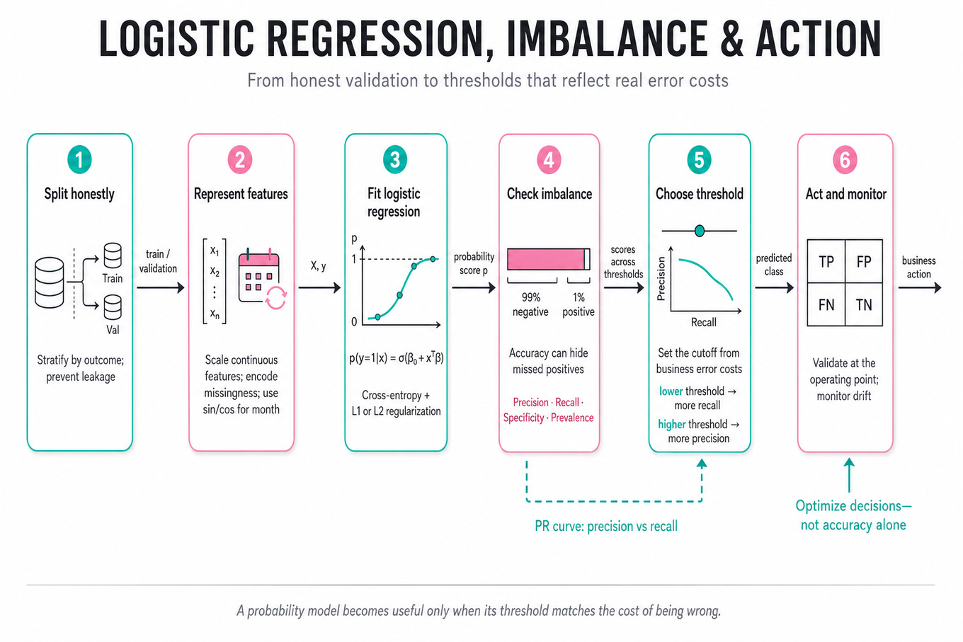
What's being tested

These questions test whether you can connect logistic regression, imbalanced classification, and decision-making under asymmetric error costs, rather than reciting model definitions. You should be able to diagnose whether poor performance comes from data leakage, feature representation, regularization, class imbalance, threshold choice, or genuine underfitting. Google cares because deployed classifiers influence user experiences and operational decisions, so a Data Scientist must select metrics, validate honestly, and translate probabilities into business actions.

Core knowledge

• Logistic regression models the positive-class probability as $p(y=1\mid x)=\sigma(\beta_0+x^\top\beta)$, where $\sigma(z)=1/(1+e^{-z})$. The log-odds are linear: $\log\frac{p}{1-p}=\beta_0+x^\top\beta$, making coefficients interpretable but limiting nonlinear interactions.

• Training usually minimizes cross-entropy loss: $-\frac{1}{n}\sum_i[y_i\log p_i+(1-y_i)\log(1-p_i)]$. It strongly penalizes confident wrong predictions and estimates probabilities well when labels, features, and regularization are appropriately specified.

• L1 regularization adds $\lambda\|\beta\|_1$ and can produce sparse coefficients, useful for many correlated or weak features; L2 regularization adds $\lambda\|\beta\|_2^2$ and usually distributes weight more smoothly. Tune $\lambda$ using leakage-safe cross-validation.

• Feature scaling is not required for tree splits, but it matters for gradient-based logistic optimization and makes regularization comparable across coefficients. Standardize continuous features, handle missingness explicitly, and encode categorical variables consistently between training and evaluation.

• Calendar variables require representation care: month encoded as integers creates a false distance between December and January. Encode cyclic seasonality as $\sin(2\pi m/12)$ and $\cos(2\pi m/12)$, or use appropriate one-hot indicators when month effects need not be smooth.

• Class imbalance makes accuracy misleading: predicting every example as negative can achieve 99% accuracy with a 1% positive rate while detecting nothing. Report the confusion matrix, prevalence, precision, recall, specificity, and metrics at an operationally meaningful threshold.

• Precision–recall curves plot precision against recall as the score threshold varies. Precision is $\frac{TP}{TP+FP}$ and recall is $\frac{TP}{TP+FN}$; average precision or AUPRC is often more informative than AUROC when positives are rare because it reflects false-positive burden among predicted positives.

• AUROC measures ranking quality across all thresholds: $\Pr(s^+>s^-)$, approximately. It can look strong with extreme imbalance even when precision is unusable, so pair it with AUPRC, prevalence, precision at a required recall, or recall at a fixed review capacity.

• Calibration asks whether predicted probabilities match observed frequencies: among cases assigned probability 0.8, roughly 80% should be positive. Use reliability diagrams, calibration slope/intercept, Brier score, or held-out calibration methods such as Platt scaling or isotonic regression.

• Threshold selection is a decision problem, not a default modeling fact. With false-positive cost $C_{FP}$ and false-negative cost $C_{FN}$, choose the threshold using expected cost, capacity, or service-level constraints; never tune it on the test set.

• Imbalance can be addressed with class-weighted loss, resampling, or thresholding. Class weights alter the optimization objective and may distort probability calibration; oversampling must occur inside each training fold, never before splitting, or duplicate examples can leak across validation data.

• Validation must match the deployment unit and time direction. Use grouped splits when multiple rows belong to one user, domain, or document, and temporal splits when future information would be unavailable at prediction time; otherwise metrics can be dramatically overstated.

• Random forests capture nonlinearities and interactions with little feature scaling, but can overfit small datasets, produce less smooth probabilities, and be difficult to interpret. Logistic regression often wins when labels are limited, effects are approximately additive, and calibrated extrapolation matters.

• Diagnose underfitting through high training and validation error, residual structure, or systematically poor performance across subgroups. Diagnose overfitting through a large train–validation gap, unstable coefficients, performance collapse under temporal or grouped validation, and improvement from stronger regularization.

Worked example

For “Identify and Fix Predictive Model Performance Gaps,” I would first clarify the target, prediction horizon, positive-class prevalence, deployment threshold, and whether the reported gap is between training and validation, segments, or time periods. I would organize the response around four pillars: audit the split and label definition for leakage, correct feature representation such as cyclical month encoding, standardize features and tune regularization, and evaluate imbalance with recall, precision, AUPRC, calibration, and threshold-specific costs. I would explicitly ask whether the model must rank cases or make a fixed action, because that determines whether ranking metrics or thresholded confusion-matrix metrics dominate. If recall is the priority, I might use class-weighted cross-entropy or select a lower threshold, while warning that this can sharply increase false positives and may require recalibration. I would compare results under a grouped or temporal holdout if repeated entities or future prediction are involved. I would close by saying that, given more time, I would inspect subgroup calibration, confidence intervals from bootstrap or repeated splits, and error examples near the selected threshold.

A second angle

For “Compute precision–recall curve on imbalanced data,” the framing shifts from debugging a model to constructing a trustworthy evaluation procedure. I would preserve continuous scores, sort examples by descending score, and compute cumulative true positives and false positives at each distinct threshold rather than evaluating only 0.5. I would emphasize that the baseline precision equals the positive prevalence, so AUPRC must be interpreted relative to that baseline and the operational cost of review. I would also distinguish average precision from trapezoidal interpolation and report a selected operating point, such as recall at a precision floor.

Common pitfalls

Pitfall: Saying “use accuracy because the model is 99% accurate” ignores prevalence and can reward an all-negative classifier. Report a confusion matrix and choose metrics tied to the action cost or capacity.

Pitfall: Treating AUROC as sufficient for rare-event detection is analytically incomplete. A model can rank positives well while producing unacceptable precision; add AUPRC and threshold-specific performance.

Pitfall: Listing class weights, SMOTE, and threshold tuning without explaining validation or calibration sounds memorized. State where each operation occurs, how the threshold is selected, and what tradeoff it creates.

Connections

An interviewer may pivot to cost-sensitive learning, probability calibration, survival or time-to-event modeling, fairness across subgroups, or drift monitoring. Be ready to distinguish population-level discrimination from subgroup reliability and from causal claims about interventions.

Further reading

• “The Precision-Recall Plot Is More Informative than the ROC Plot When Evaluating Binary Classifiers on Imbalanced Datasets” — Davis and Goadrich’s classic comparison of ROC and precision–recall evaluation.

• “Predicting Probabilities with Supervised Learning” — Practical treatment of calibration and probability quality.

• The Elements of Statistical Learning, Hastie, Tibshirani, and Friedman — Chapters 4, 7, and 9 for logistic regression, model assessment, and additive/nonlinear methods.

Practice questions

Focus area — You explicitly selected time-series forecasting and anomaly detection, and ML is 2/5; practice Google-scale metric monitoring and incident detection.

What's being tested

A strong candidate must translate an ambiguous product-monitoring request into a precise time-series target, forecast horizon, anomaly definition, and decision policy. The interviewer is probing whether you can distinguish genuine product changes from seasonality, trend, data-quality artifacts, and expected experimentation effects. For a Data Scientist, Google cares about this because trustworthy anomaly detection informs incident response, product launches, experimentation interpretation, and prioritization—not merely model accuracy.

Core knowledge

• Metric specification comes first: define the numerator, denominator, population, timestamp semantics, aggregation window, and alert consumer. “Search success” might mean query-level success rate, user-level next-action rate, or a ratio of aggregated counts; these have different variance and business meaning.

• Time-series decomposition separates level, trend, seasonality, and residual:
  $y_t = T_t + S_t + R_t$
  or, for multiplicative behavior, $y_t = T_tS_tR_t$. Use additive structure when seasonal amplitude is stable and multiplicative or log-scale structure when volatility grows with the metric level.

• Seasonality may be daily, weekly, annual, holiday-driven, or event-driven. A Monday-to-Sunday comparison is often more meaningful than a prior-day comparison. Include calendar features such as day of week, hour, holidays, school breaks, and known launches, but avoid encoding future information unavailable at prediction time.

• Baselines are essential and often competitive: seasonal naïve forecasting predicts $y_t$ from the same weekday and hour in the prior week; a robust baseline can use the median of the last $k$ comparable periods. Compare every sophisticated model against these before claiming improvement.

• Forecasting models span exponential smoothing, ARIMA/SARIMA, dynamic regression, gradient-boosted trees, and global neural models. Prophet-style trend-plus-seasonality models are convenient, while XGBoost with lag, rolling, and calendar features can perform well across many related product metrics; complexity should match data volume and horizon.

• Anomaly detection should operate on forecast errors or prediction intervals, not raw values alone. If $\hat y_t$ is the expected value, define the residual $e_t=y_t-\hat y_t$ and alert when $e_t$ exceeds a calibrated bound, such as
  $|e_t| > z_{1-\alpha/2}\hat\sigma_t.$
  Use robust scale estimates such as MAD when residuals contain outliers.

• Prediction intervals express uncertainty: a point forecast can be accurate on average while still producing poor alert boundaries. Evaluate empirical coverage—whether a nominal 95% interval contains roughly 95% of future observations—and interval width; narrow, under-covering intervals create noisy alerts.

• Backtesting must respect temporal order. Use rolling-origin evaluation: train through time $t$, forecast the next horizon, advance the cutoff, and repeat. Random cross-validation leaks future patterns and typically overstates performance, especially when trends, launches, or autocorrelation exist.

• Metrics should match the operational goal. Use MAE or RMSE for point forecasts, WAPE or MASE for scale-normalized comparisons, and pinball loss for quantiles. For anomaly alerts, measure precision, recall, time-to-detection, alert volume, and false alerts per metric-day; “accuracy” is usually misleading under extreme class imbalance.

• Robustness matters more than average error. Segment performance by geography, device, traffic volume, product surface, and forecast horizon. Check behavior around holidays, traffic spikes, zeros, missing intervals, denominator changes, and metric-definition changes; a model that wins globally may fail for a high-value segment.

• Causal interpretation is separate from detection. An anomaly identifies an unusual change, not its cause. Diagnose with metric decomposition, cohort slices, funnel steps, experiment assignments, and correlated product metrics; use controlled experiments or quasi-experimental methods before claiming that a feature caused the movement.

• Alert policy should reflect cost asymmetry and persistence. Require two or more consecutive breaches, use hysteresis to prevent repeated open/close alerts, and prioritize by estimated user impact. A practical score can combine standardized deviation, affected volume, duration, and business criticality rather than ranking solely by statistical significance.

Worked example

Design a forecasting and anomaly-detection approach for a Google product metric is a representative framing for this topic. In the first 30 seconds, clarify the metric definition, sampling frequency, forecast horizon, alert latency, expected anomaly labels, and whether the goal is incident detection, capacity planning, or experiment monitoring. State an assumption such as hourly query-success rate for a major product surface, with alerts needed within two hours and strong weekday seasonality. Organize the answer around four pillars: a seasonal-naïve baseline, a forecasting model with calendar and lag features, residual-based prediction intervals, and an evaluation and diagnosis plan. Explicitly separate metric movement from root-cause analysis by proposing cohort and funnel slices after an alert fires. One key tradeoff is sensitivity versus alert fatigue: tighter intervals detect smaller regressions but can overwhelm responders, so calibrate thresholds against historical incidents and a false-alert budget. Close by saying that, with more time, you would validate subgroup coverage, test holiday and launch robustness, and estimate the user impact of missed versus spurious alerts.

A second angle

A different framing is detecting anomalies in a sparse, low-volume metric across many countries. Here, raw percentage changes are unstable because a small denominator can create enormous swings, so model numerator and denominator jointly or use binomial or beta-binomial uncertainty. Partial pooling or hierarchical models can borrow strength across related countries while preserving meaningful local deviations. The operational goal may also favor ranking the most credible anomalies rather than producing a binary alert for every series.

Common pitfalls

Pitfall: Treating every deviation from the previous hour as an anomaly ignores daily and weekly seasonality, trend, and changing variance. Use a seasonal baseline or forecast residual and validate its interval coverage.

A tempting analytical mistake is to report lower RMSE as proof that the alerting system is better. Forecast accuracy and detection quality are different objectives; evaluate precision, recall, detection delay, alert volume, and business impact separately.

Pitfall: Saying “the model will identify the root cause” overclaims what forecasting can do. Detection should trigger structured segmentation, funnel analysis, experiment checks, and causal investigation.

A communication mistake is jumping immediately to ARIMA, Prophet, or a neural model without defining the metric and decision. Interviewers generally reward an explicit target, horizon, baseline, validation design, and alert policy before model sophistication.

A depth mistake is ignoring uncertainty and data sparsity. Point forecasts alone cannot set reliable thresholds, and a 5% change in a high-volume count is not statistically equivalent to a 5% change in a tiny cohort.

Connections

An interviewer may pivot to causal inference, experiment analysis, metric design, or hierarchical modeling. They may also ask about change-point detection, multiple-testing correction across thousands of monitored metrics, or how to distinguish product regressions from measurement changes.

Further reading

• Forecasting: Principles and Practice — Hyndman and Athanasopoulos’s practical treatment of decomposition, backtesting, intervals, and forecast evaluation.

• S. S. Vallis, J. Hochenbaum, and A. Kejariwal, “A Novel Technique for Long-Term Anomaly Detection in the Cloud” — introduces the Seasonal Hybrid ESD approach used for robust seasonal anomaly detection.

• S. Aminikhanghahi and D. J. Cook, “A Survey of Methods for Time Series Change Point Detection” — useful taxonomy for distinguishing isolated anomalies from persistent regime changes.

Practice questions

Behavioral & Leadership

Focus area — Behavioral is 2/5, and you selected stakeholder alignment, conflict, influence, executive communication, ambiguity, prioritization, and mentoring.

What's being tested

Interviewers are probing your ability to lead through data ambiguity: clarify fuzzy requests, pick defensible assumptions, quantify trade-offs, and influence non-technical stakeholders to a data-driven decision. They expect a Data Scientist to combine statistical judgment, experiment design, and concise storytelling so business partners can act. Google cares because ambiguous, cross-functional problems are common and a DS must translate analysis into measurable outcomes and repeatable plans.

Core knowledge

• Problem framing: Always start with the decision to be made, the primary business metric (e.g., DAU, revenue per user), and the time horizon; this orients analysis and trade-offs immediately.

• Causal vs observational: Know when observational analyses can support decisions and when only an A/B test (randomized experiment) gives causal inference; articulate confounders and use causal diagrams (DAGs) to explain them.

• Metric design & guardrails: Define a primary metric, at least one quality guardrail (e.g., error rate, latency), and interpretation rules (min detectable effect, directionality, loss tolerance).

• Power & sample-size: Use the standard two-sample formula: $n \approx \left(\frac{Z_{1-\alpha/2}+Z_{1-\beta}}{\delta/\sigma}\right)^2$ Explain inputs: effect size $\delta$, baseline variance $\sigma^2$, Type I/II errors.

• Effect size vs significance: Distinguish statistical significance (p-value) from practical significance (business-impact size), and always report confidence intervals for effect estimates.

• Multiple comparisons & heterogeneity: Account for subgroups and multiple metrics with Bonferroni or hierarchical testing; plan for heterogeneous treatment effects (HTE) and pre-specify subgroup analyses.

• Quick evidence vs rigor trade-off: Lay out the speed/precision trade: observational signal gives fast directional insight; short experiments reduce variance at cost of slower deployment. Quantify uncertainty (CI width) to justify speed.

• Communicating to non-technical partners: Use one-sentence conclusions, one chart (effect with CI), and one recommended action. Translate statistical jargon into business terms (e.g., "expected revenue lift of $X/month, 95% CI").

• Handling pushback: Use small pilots or sequential testing to de-risk; predefine stopping rules or Bayesian priors to update stakeholders continuously.

• Experimentation pitfalls: Watch for peeking, non-random assignment, instrumentation gaps, and SUTVA violations (spillovers); have logging/QA checks and monitor guardrail metrics.

Tip: Prepare a one-slide "Decision Brief": question, recommended action, metric impact (with CI), key risks, next steps.

Worked example — "Demonstrate leadership in data ambiguity"

First 30 seconds: ask clarifying questions: "What decision will this analysis support?", "Who will act on it?", "What are acceptable trade-offs or guardrails?" Declare assumptions you must make (e.g., treatment assignment, user population). Skeleton answer pillars: (1) quick diagnostic to surface possible causes (metric decomposition), (2) hypothesis-driven tests (observational checks + targeted A/B test), (3) quantified recommendation with risk mitigation (pilot, rollback criteria). Flag a concrete trade-off: doing an immediate observational segmentation may suggest a high uplift but could be confounded; recommend a small randomized pilot limited to 10% of traffic to validate directionally in 2 weeks, showing how sample-size calculation yields required N. Close by saying, "If I had more time I'd instrument additional covariates to explain heterogeneity and run a pre-registered subgroup analysis; with partners I’d schedule a two-week pilot and a post-mortem to refine the rollout plan."

A second angle — "Describe Overcoming Challenges and Persuading Non-Data Colleagues"

In this scenario the constraint is persuasion under skepticism and tight timelines. Start by translating the ask into a decision and headline metric, then present a compact evidence package: one clear visualization (treatment effect with CI), one robustness check (difference-in-differences or placebo window), and one small recommended experiment. Use narrative: "Here’s the potential upside, here’s the risk, here’s a low-cost pilot that will resolve it." When stakeholders resist randomized tests, propose a phased rollout with defined success criteria and automatic rollback. Emphasize empathy: validate their concerns, show how the plan protects revenue/UX, and propose concrete milestones so they feel control over risk.

Common pitfalls

Pitfall: Analytical mistake — Over-interpreting correlations. Running many subgroup checks and presenting the largest observed lift without correcting for multiple comparisons will mislead stakeholders; always pre-specify or adjust.

Pitfall: Communication mistake — Jargon and detail overload. Launching into p-values, standard errors, and model hyperparameters without a one-line recommendation loses non-technical partners; lead with the decision and impact first.

Pitfall: Depth mistake — No trade-offs quantified. Saying "we should run an experiment" without a sample-size, timeline, or guardrail plan makes guidance unusable. Always quantify time-to-confidence, cost, and potential downside.

Connections

This skillset naturally pivots to experiment design (power, variants), metric design (sensitivity, guardrails), and model evaluation (deployment risk, offline vs. online metrics). Interviewers might follow up into sequential testing, causal identification strategies, or A/B test infrastructure questions.

Further reading

• Practical Guide to Controlled Experiments on the Web (Kohavi et al.) — essential on experiment design pitfalls and trustworthy online experiments.

• Evan Miller’s A/B Testing Guide — pragmatic explanations of power, sample size, and sequential testing for product experiments.

Practice questions