Microsoft Machine Learning Engineer Interview Prep Guide

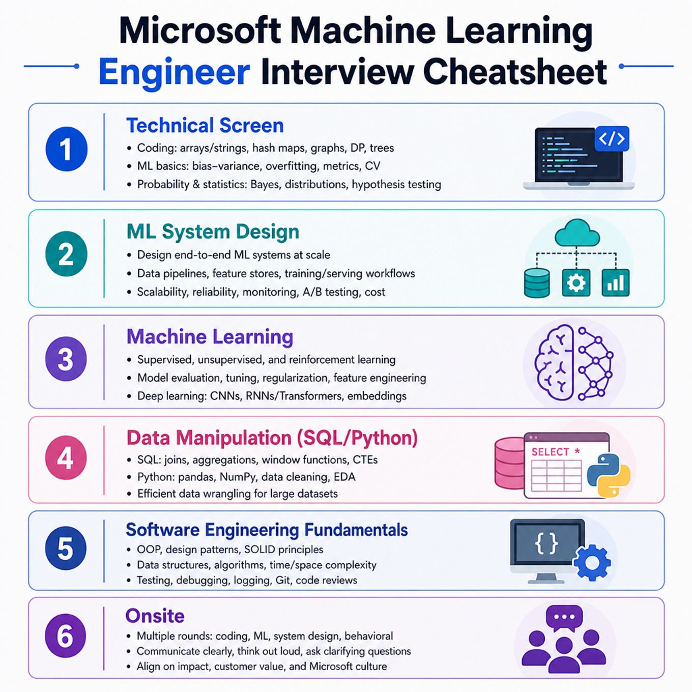
Focus most on production ML system design, RAG/retrieval, transformers/LLM internals, ranking/recommenders, and serving/monitoring because you self-rated ML System Design 1/5 and called out production ML and LLM internals as weak. Since no area has strong solved-history signals, the lightest review bucket is graph BFS plus research-adjacent k-means, bias-variance, and basic coding patterns. The Microsoft-specific emphasis is enterprise RAG/search, Responsible AI groundedness, Azure-style safe rollout/observability, and recommender-style ranking for large-scale products. With 30 days, spend roughly the first half rebuilding system-design depth, the second half alternating Python/NumPy implementation, evaluation metrics, recommender coverage, and mock interviews.

Technical Screen — 69 min

ML System Design

• RAG And Agentic Tool Use (Focus) — covered in depth under Onsite below.

• Large Language Models (Focus) — covered in depth under Onsite below.

• Search Ranking And Indexing (Focus) — covered in depth under Onsite below.

• Recommender Systems Ranking And CTR (Focus) — covered in depth under Onsite below.

Machine Learning

• PyTorch And NumPy Training Loops (Focus) — covered in depth under Onsite below.

• Time Series Modeling And Forecasting (Focus) — covered in depth under Onsite below.

Data Manipulation (SQL/Python)

Focus area — You specified Python plus NumPy/pandas and viewed data-manipulation content; emphasize joins, groupbys, vectorization, missing values, and feature-table construction.

What's being tested

This tests vectorized data manipulation with pandas and NumPy: filtering, joining, reshaping, aggregation, missing-value handling, and array broadcasting. The candidate must choose idiomatic operations over Python loops, preserve row alignment, avoid leakage or unintended mutation, and reason about time and memory costs in an ML pipeline.

Patterns & templates

• Boolean filtering with df.loc[mask, columns]; combine conditions with & and |, parenthesize each expression, and use .isin() for membership.

• Group aggregation with df.groupby(keys, observed=True).agg(...); named aggregations improve readability, while .transform() preserves original row count for features.

• Safe joins with pd.merge(..., how="left", validate="many_to_one"); inspect key uniqueness to prevent accidental Cartesian row explosions.

• Missing values using .isna(), .fillna(), and .dropna(); fit imputers on training data only, then reuse them for validation and serving.

• Vectorized NumPy operations use broadcasting and functions such as np.where, np.clip, np.nanmean, and np.select; avoid row-wise .apply() when arrays suffice.

• Reshaping with pivot_table, melt, and stack; explicitly define aggregation when duplicate index-column pairs exist.

• Performance favors columnar operations, categorical keys, and selective columns; estimate memory because a 10M-row merge can exceed available RAM.

Common pitfalls

Pitfall: Using df["flag"] == True or chained indexing can create ambiguous behavior; use .loc and explicit boolean expressions.

Pitfall: groupby().mean() silently excludes missing values, while joins may duplicate records; validate row counts and null rates afterward.

Pitfall: axis=0 operates down rows and axis=1 across columns; confirm shapes before relying on broadcasting.

Practice these

The practice cards below cover the canonical variants—solve all of them and time yourself.

Practice questions

Software Engineering Fundamentals

• Robust Python Components And API Failure Handling (Focus) — covered in depth under Onsite below.

Onsite — 77 min

ML System Design

Focus area — You selected RAG, retrieval, agentic AI, LangChain, chunking, reranking, and ANN topics; this is a core Microsoft enterprise-search pattern.

What's being tested

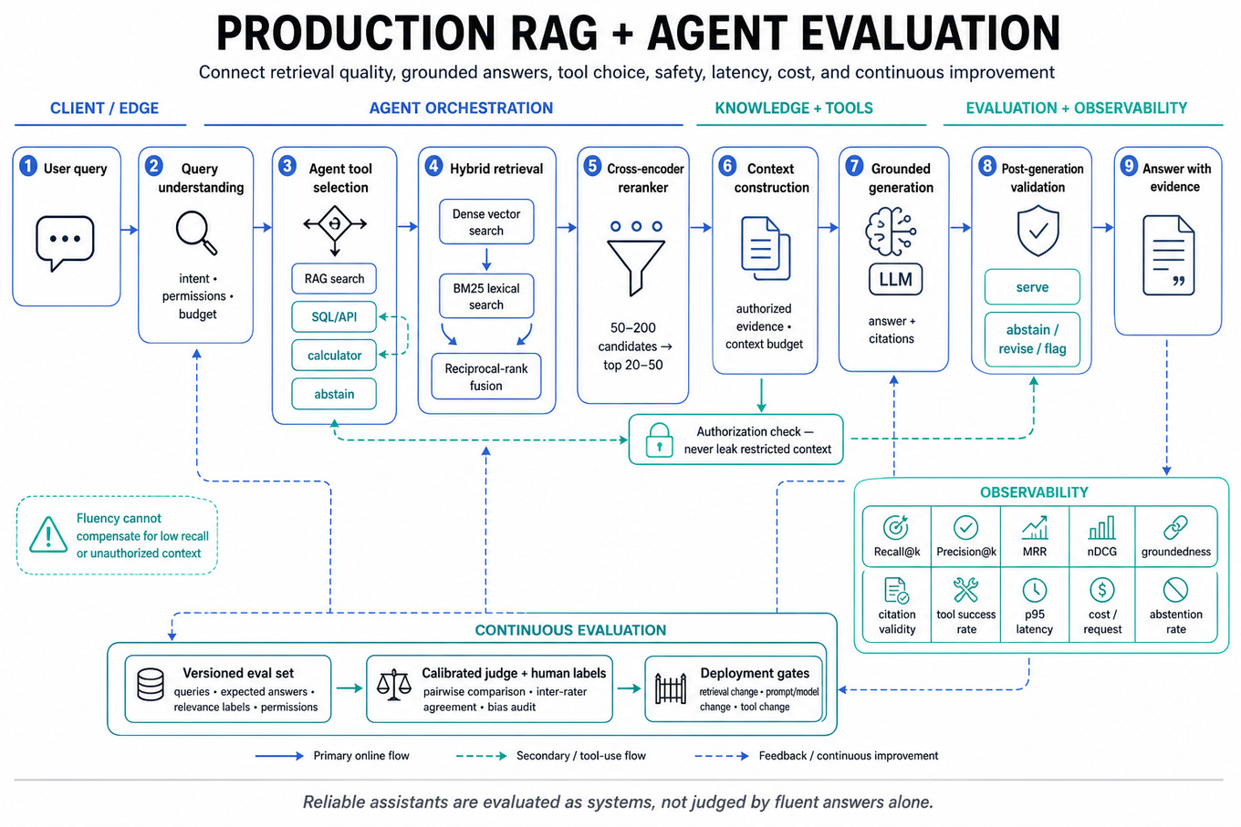
These interviews test whether you can turn an LLM prototype into a measurable, reliable production ML system rather than merely describe embeddings and prompts. You must connect retrieval quality, generation groundedness, agentic tool selection, latency, cost, safety, and continuous improvement into one evaluation loop. Microsoft cares because enterprise assistants operate over changing, permissioned knowledge and must provide evidence-backed answers with predictable behavior. The interviewer is probing for explicit metrics, versioned evaluation data, calibrated judges, failure diagnosis, deployment gates, and monitoring tied to model and retrieval changes.

Core knowledge

• RAG architecture separates query understanding, retrieval, reranking, context construction, generation, and post-generation validation. Treat each stage as observable and replaceable; a fluent answer cannot compensate for low retrieval recall or unauthorized context.

• Hybrid retrieval combines dense vector search with lexical methods such as BM25. Dense embeddings capture semantic similarity, while lexical retrieval preserves exact identifiers, acronyms, error codes, and names; reciprocal-rank fusion is a practical baseline before learned reranking.

• Retrieval evaluation should measure Recall@k, Precision@k, MRR, and nDCG against versioned relevance labels. Also measure answer-level groundedness: retrieved passages must contain sufficient evidence, not merely be topically similar to the query.

• Rerankers such as cross-encoders improve precision by scoring query-document pairs jointly, but add latency and compute cost. A common design retrieves 50–200 candidates cheaply, reranks the top 20–50, then supplies only the best evidence within the context budget.

• Grounded generation requires citation or claim verification, not just a “retrieval succeeded” flag. For claims $c_i$, a simple groundedness estimate is $\frac{1}{n}\sum_i \mathbf{1}[\text{evidence supports }c_i]$; unsupported claims should be abstained, revised, or flagged.

• LLM-as-a-judge is useful for semantic quality but is biased by verbosity, position, and model style. Calibrate it against human labels, use pairwise comparisons where appropriate, report inter-rater agreement, and periodically audit difficult, adversarial, and minority-language examples.

• Evaluation datasets need query, expected answer or claims, relevant evidence, permitted tools, and policy labels. Version them with corpus snapshots, prompts, model IDs, retriever configuration, and judge configuration so regressions are attributable and reproducible.

• Agentic tool use should be modeled as a constrained policy: select a tool, validate arguments, execute with authorization and timeout, inspect the result, and either continue or answer. Use strict schemas, allowlists, idempotency where applicable, bounded steps, and explicit termination conditions.

• Tool-selection metrics include tool-call precision, successful execution rate, argument validity, unnecessary-call rate, task completion, and recovery from tool failures. A correct final answer with an unsafe or unauthorized intermediate call is still a system failure.

• Online monitoring combines quality proxies and operational signals: groundedness, citation coverage, abstention rate, user correction rate, task success, tool errors, token cost, p50/p95/p99 latency, and rate of retrieval-empty or context-overflow events. Segment by tenant, intent, language, and permission scope.

• Improvement loops should isolate one change at a time when possible: corpus/chunking, embedding model, retrieval, prompt, generation model, or tool policy. Run offline regression gates first, shadow or canary traffic next, and roll back automatically when guardrail or quality thresholds regress.

• Distribution shift and freshness are distinct problems: drift in query or document distributions can degrade retrieval, while stale indexes produce outdated answers even when embeddings remain well calibrated. Track freshness, document-version coverage, embedding drift, and performance on newly sampled queries.

Worked example: Design an Evaluation and Improvement Loop for a Production LLM Application

A strong candidate first clarifies the application’s users, supported tasks, knowledge freshness requirements, latency and cost budgets, acceptable risk, and whether answers must include citations or tool actions. They would declare that quality is multi-dimensional: retrieval relevance, groundedness, correctness, completeness, safety, task success, and user-perceived helpfulness. The answer can then be organized around four pillars: a versioned evaluation set, component-level offline metrics, calibrated end-to-end evaluation, and production monitoring with a gated improvement loop. They would compare retrieval labels and Recall@k with claim-level groundedness and judge or human ratings, rather than relying on one overall LLM score. A key tradeoff is judge-model cost versus evaluation coverage: use a cheaper calibrated judge for broad regression testing and humans for a stratified, high-risk sample. They would version prompts, models, corpus snapshots, retriever settings, and tool policies to make failures reproducible. Deployment would use offline thresholds followed by shadow traffic, canaries, and rollback on quality, safety, latency, or cost regressions. If they had more time, they would add slice-based analysis for tenants, languages, intents, adversarial prompts, and newly introduced documents.

A second angle

For Design a RAG system with agentic tools, the same evaluation discipline must cover the trajectory, not only the final response. The candidate should distinguish retrieval failures, wrong-tool selection, invalid arguments, authorization failures, tool-result interpretation errors, and unsupported synthesis. A useful design constrains tool calls with schemas and permissions, then measures success rate, unnecessary calls, recovery rate, step count, latency, and cost alongside answer groundedness. The central framing shifts from “does the model answer well?” to “does the policy complete the task safely and efficiently under bounded autonomy?”

Common pitfalls

Pitfall: Treating retrieval hit rate or cosine similarity as answer quality. Similarity can return semantically related but non-authoritative passages; pair retrieval metrics with evidence sufficiency, claim entailment, citation correctness, and end-to-end task success.

Pitfall: Saying “we monitor user feedback” without defining an evaluation protocol. Explain how explicit ratings, corrections, escalations, sampled traces, and judge scores are labeled, segmented, calibrated, and converted into retraining or rollback decisions.

Pitfall: Hand-waving agent behavior as “the LLM decides which tool to call.” A stronger answer specifies tool schemas, authorization boundaries, retries, timeouts, maximum steps, idempotency, failure recovery, and what happens when evidence or tool results are insufficient.

Connections

The interviewer may pivot to model serving, feature and data versioning, online/offline parity, drift detection, responsible AI, or A/B and canary experimentation. Be ready to explain how evaluation artifacts and telemetry connect to deployment gates and rollback mechanisms.

Further reading

• Retrieval-Augmented Generation for Knowledge-Intensive NLP Tasks — foundational RAG architecture and motivation.

• RAGAS: Automated Evaluation of Retrieval Augmented Generation — practical framework for evaluating retrieval and grounded generation.

• Toolformer: Language Models Can Teach Themselves to Use Tools — foundational perspective on tool-use learning and execution traces.

Practice questions

Focus area — You called transformers/LLM internals rusty and ML system design is 1/5; emphasize attention, context limits, latency, safety, and Microsoft Responsible AI.

What's being tested

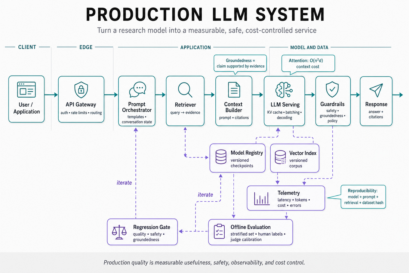
These prompts test whether you can turn an LLM from a research artifact into a measurable, deployable, and improvable production component. The interviewer is probing for transformer fundamentals, evaluation design, groundedness and safety measurement, model-serving tradeoffs, and disciplined iteration rather than vague claims that a larger model is “better.” Microsoft cares because production assistants must remain useful, safe, observable, and cost-controlled across changing prompts, models, retrieval corpora, and user populations.

Core knowledge

• Transformer architecture uses token embeddings plus positional information, then repeated self-attention and feed-forward blocks. For sequence length $n$ and hidden dimension $d$, standard attention has approximately $O(n^2d)$ compute and memory pressure, making long-context serving expensive.

• Scaled dot-product attention is
  $\operatorname{Attention}(Q,K,V)=\operatorname{softmax}\left(\frac{QK^\top}{\sqrt{d_k}}+M\right)V.$
  Causal masking sets future-token logits to $-\infty$; padding masks prevent attention to nonexistent tokens.

• Autoregressive decoding generates one token at a time. KV caching stores prior keys and values so each new token attends without recomputing the full prefix; it improves latency but increases memory roughly with batch size, layers, sequence length, and head dimension.

• Decoding strategy changes both quality and reproducibility: greedy decoding is deterministic, beam search is more useful for constrained generation, and temperature/top-$p$ sampling improves diversity. Evaluation must fix seeds or report confidence intervals when comparing stochastic versions.

• Offline evaluation should use a versioned, stratified dataset containing representative requests, adversarial cases, long contexts, multilingual examples, and known regressions. Track model, prompt, retrieval configuration, evaluator version, and dataset hash so results are reproducible.

• LLM-as-a-judge can score relevance, correctness, style, or safety, but judge scores require calibration against human labels. Measure agreement such as Cohen’s $\kappa$ or Spearman correlation, test position and verbosity bias, and retain human review for high-impact decisions.

• Groundedness asks whether each claim is supported by supplied evidence, not merely whether the answer sounds plausible. A practical sentence-level score is
  $\text{groundedness}=\frac{\#\text{supported factual claims}}{\#\text{factual claims}},$
  with abstention or citation requirements when support is absent.

• Retrieval-augmented generation (RAG) quality decomposes into retrieval recall, context precision, answer faithfulness, and answer usefulness. Diagnose retrieval separately from generation: a correct answer is impossible when the required evidence is not retrieved, while irrelevant context can induce distraction or contradictions.

• Online monitoring should combine quality proxies and operational metrics: groundedness, refusal rate, task success, user feedback, token usage, throughput, p50/p95/p99 latency, timeout rate, and safety-violation rate. Segment by language, task, tenant, model version, and traffic cohort to expose localized regressions.

• Drift monitoring covers input, retrieval, and output distributions. Track embedding-distance or population-stability changes, prompt-length shifts, retrieval hit rates, citation coverage, and judge-score distributions; alert thresholds should be calibrated to false-positive cost rather than chosen arbitrarily.

• Safe deployment uses shadow traffic, canaries, feature flags, automatic rollback, rate limits, content filtering, prompt-injection defenses, and least-privilege tool access. Canary decisions should use minimum sample sizes and guardrails for safety, latency, cost, and quality—not only average user preference.

• Serving optimization balances quality against cost and latency through quantization, batching, continuous batching, speculative decoding, prompt-prefix caching, smaller routing models, and distillation. Quantization can reduce memory and improve throughput, but validate degradation separately for rare languages, long contexts, tool calls, and safety behavior.

Worked example

For Design an Evaluation and Improvement Loop for a Production LLM Application, I would first clarify the application’s task, user population, risk level, latency and cost targets, available feedback, and whether answers must cite an approved knowledge base. I would state an assumption such as a RAG assistant where correctness and groundedness matter more than stylistic preference. I would organize the design around four pillars: a versioned evaluation corpus, calibrated offline evaluators, production monitoring with segmented slices, and a controlled improvement and rollback loop. The offline set would include golden answers or evidence labels, adversarial prompts, historical failures, and new samples from production, while separating development, validation, and final holdout data. I would compare prompt, model, retriever, and chunking versions using task success, groundedness, citation correctness, refusal quality, latency, and cost. A key tradeoff is using an LLM judge for scale versus human labels for validity: I would calibrate the judge, estimate disagreement, and route uncertain or high-risk examples to humans. Online, I would canary changes and require no regression on safety and latency guardrails even if aggregate quality improves. If I had more time, I would add active learning to prioritize uncertain failures and analyze whether improvements generalize across languages, tenants, and long-tail intents.

A second angle

For Explain Transformers and deploy an LLM safely, the same evaluation mindset is applied earlier, at the model-serving boundary. The candidate should connect causal masking, KV-cache memory, batching, quantization, and decoding choices to measurable p99 latency, throughput, cost, and response quality. The framing shifts from “how do we improve an existing application loop?” to “what architecture and deployment controls make the model reliable under production load?” A strong answer still defines quality and safety gates before selecting serving optimizations. It should explicitly test that compression or speculative decoding does not create regressions in refusal behavior, factuality, or rare but high-severity prompts.

Common pitfalls

Pitfall: Treating lexical overlap such as BLEU or ROUGE as a sufficient hallucination metric is tempting but wrong: a fluent answer can match reference wording while contradicting the evidence. Pair task metrics with claim-level entailment, citation verification, human labels, and retrieval diagnostics.

Pitfall: Saying “we monitor quality” without naming an instrumented metric, slice, threshold, or response action sounds non-operational. State an example such as: “If groundedness drops by 5% for finance queries in a canary, halt rollout, inspect retrieval misses, and automatically route traffic to the previous version.”

Pitfall: Recommending an LLM judge as objective ground truth ignores evaluator bias, prompt sensitivity, and correlated model errors. Explain calibration against humans, judge versioning, disagreement sampling, and why high-risk cases require deterministic checks or manual review.

Connections

The interviewer may pivot to RAG retrieval evaluation, responsible AI and red teaming, **model compression and GPU serving, or A/B testing with sequential monitoring. Be ready to connect each to offline/online parity, slice-level metrics, and rollback criteria.

Further reading

• Attention Is All You Need — the original Transformer architecture and attention formulation.

• HELM: Holistic Evaluation of Language Models — broad, scenario-based evaluation across accuracy, robustness, fairness, and efficiency.

• RAGAS: Automated Evaluation of Retrieval Augmented Generation — metrics and methodology for separating retrieval and generation quality.

Practice questions

Focus area — Your recommender request maps to ranking, candidate generation, calibration, and freshness; emphasize search/ranking as the closest base concept.

What's being tested

These designs test whether you can turn retrieval and ranking requirements into a production ML system with clear boundaries between candidate generation, feature computation, model serving, and evaluation. The interviewer is probing for practical knowledge of inverted indexes, vector retrieval, learning-to-rank, offline/online feature parity, latency budgets, and safe deployment. Microsoft cares because search and enterprise retrieval must serve large, heterogeneous corpora with low latency while remaining relevant, fresh, explainable, and robust to distribution shift.

Core knowledge

• An inverted index maps normalized terms to documents and supports lexical retrieval through BM25:
  $score(D,Q)=\sum_{t\in Q}IDF(t)\frac{f(t,D)(k_1+1)}{f(t,D)+k_1(1-b+b|D|/\overline{|D|})}$. It handles exact identifiers and rare terms well.

• Dense retrieval represents queries and documents as embeddings and searches nearest neighbors using cosine similarity or inner product. ANN structures such as HNSW and IVF-PQ trade recall for latency and memory; measure recall@K before optimizing index parameters.

• Hybrid retrieval combines lexical and semantic candidates because embeddings can miss exact product names, SKUs, or security-sensitive terms. Fuse normalized scores with weighted blending or reciprocal rank fusion, then deduplicate documents before reranking.

• Separate candidate generation from reranking. Retrieve hundreds or thousands of candidates using cheap indexes, then apply a heavier model such as LightGBM, XGBoost, or a cross-encoder to the top 50–500 under the request’s latency budget.

• A learning-to-rank model can use pointwise, pairwise, or listwise objectives. Typical features include BM25 score, semantic similarity, field matches, freshness, price, availability, popularity, and query-document interaction terms; avoid features unavailable at serving time.

• Define labels carefully: clicks are noisy and position-biased, while purchases or successful answers are delayed but stronger. Use graded relevance judgments where possible, and consider inverse propensity weighting when learning from displayed rankings.

• Evaluate retrieval with Recall@K, MRR, and nDCG@K; evaluate business outcomes with conversion or successful-task rate. For graded relevance,
  $DCG@K=\sum_{i=1}^{K}\frac{2^{rel_i}-1}{\log_2(i+1)}$, while online metrics require guardrails for latency, zero-result rate, and abandonment.

• Design offline/online parity for tokenization, normalization, embedding versions, feature transformations, and filtering rules. Version the model, feature definitions, and index together; otherwise, a correct offline score can conceal serving-time mismatches.

• Treat the index as a versioned model-serving artifact: build a new snapshot or shard generation, validate document counts and retrieval recall, then atomically switch an alias or routing pointer. Support rollback, partial rebuilds, and compatibility between index and embedding model.

• Establish a latency budget across query understanding, lexical retrieval, ANN search, feature lookup, reranking, and response assembly. Parallelize independent retrieval paths, cap candidate counts, cache repeated queries, and monitor p50, p95, and p99 rather than only averages.

• Drift monitoring should cover query distributions, language and category mix, embedding norms, candidate-set overlap, feature null rates, score distributions, and relevance metrics. A rising zero-result rate or falling ANN recall may indicate index freshness or model drift rather than ranking failure.

• For RAG, retrieve chunks with document-level permissions and return provenance. Enforce authorization before generation, preserve source identifiers through reranking, and test groundedness, citation correctness, prompt-injection resistance, and answer quality—not merely top-k similarity.

Worked example: Design a Product Search System

For Design a Product Search System, I would first clarify catalog size and update rate, supported languages, query types, p95/p99 latency, personalization requirements, and whether availability and authorization must be real-time. I would declare an initial target such as lexical-plus-vector candidate retrieval, a sub-200 ms p95 budget, and ranking quality measured offline before online experimentation. I would organize the answer around four pillars: document and embedding representation, hybrid candidate generation, feature-based reranking, and versioned serving and monitoring. I would describe model training from query–product interactions with position-bias-aware labels, and enforce identical transformations in training and serving. A key tradeoff is index freshness versus retrieval efficiency: near-real-time updates improve inventory correctness, while immutable snapshots make validation, rollback, and cache behavior safer. I would explicitly separate the MLE-owned model and index contracts from upstream catalog event production, while defining freshness and completeness checks at the interface. I would close by saying that with more time I would quantify shard sizing, failure behavior, multilingual evaluation, and an online experiment plan with guardrail metrics.

A second angle

For Design a RAG system with agentic tools, the same retrieval principles apply, but relevance is constrained by enterprise permissions, document freshness, chunk granularity, and answer grounding rather than product conversion. The architecture should combine metadata and ACL filtering with lexical and vector retrieval, followed by reranking and source-preserving context assembly. Agentic tool calls add a policy layer: validate tool arguments, constrain retrieval scope, detect prompt injection, and prevent unauthorized data from entering the context. Evaluation must include retrieval recall, citation correctness, grounded answer rate, tool success rate, and end-to-end latency.

Common pitfalls

Pitfall: Treating nDCG or click-through rate as sufficient evidence of quality. Ranking metrics can improve while inventory correctness, latency, or successful task completion deteriorates; pair relevance metrics with operational and user-value guardrails.

Pitfall: Giving a data-platform design instead of an MLE design. Describing partition tuning, stream retries, or warehouse schemas misses the role; focus on index/model artifacts, feature contracts, serving parity, deployment, and monitoring.

Pitfall: Saying “use embeddings and a transformer” without a candidate-count or latency plan. A stronger answer specifies lexical versus ANN recall, reranker cutoff, model quantization or distillation, timeout behavior, and how quality is measured after each stage.

Connections

The interviewer may pivot to feature stores, model deployment and canarying, counterfactual evaluation for biased feedback, or concept drift and retraining triggers. Be ready to connect retrieval quality to distributed serving constraints without drifting into data-engineering ownership.

Further reading

• Learning to Rank for Information Retrieval — comprehensive treatment of ranking objectives, features, and evaluation.

• The Probabilistic Relevance Framework: BM25 and Beyond — foundations of lexical scoring and term-based retrieval.

• Efficient and Robust Approximate Nearest Neighbor Search Using Hierarchical Navigable Small World Graphs — practical foundations for HNSW vector indexes.

Practice questions

Focus area — You explicitly asked for recommender coverage; focus on two-tower retrieval, collaborative signals, CTR ranking, calibration, diversity, and cold-start tradeoffs.

What's being tested

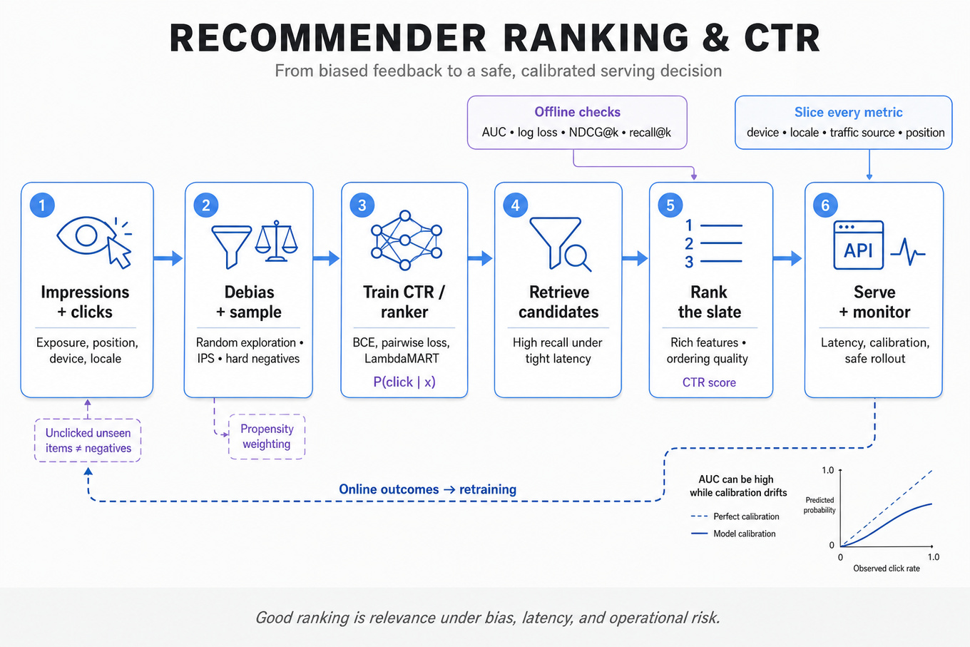
This topic tests whether you can build and operate a learning-to-rank system whose predictions remain useful under real serving constraints. The interviewer is probing your understanding of CTR modeling, biased feedback data, offline-to-online evaluation, feature freshness, latency, and deployment safety. Microsoft cares because ranking models directly influence high-volume user experiences, and a small modeling or serving regression can affect both relevance and system cost at large scale.

Core knowledge

• Ranking architecture usually has multiple stages: candidate retrieval, lightweight filtering, and a more expensive ranker. Retrieval optimizes recall under tight latency; ranking optimizes ordering quality using features unavailable or too costly for millions of candidates.

• CTR prediction estimates $P(\text{click}\mid x)$, commonly with logistic regression, LightGBM, XGBoost, deep cross networks, or transformer-based models. Binary cross-entropy is typical:
  $-\frac{1}{N}\sum_i[y_i\log p_i+(1-y_i)\log(1-p_i)]$

• Pairwise and listwise ranking losses optimize ordering rather than isolated probabilities. LambdaMART approximates changes in NDCG; pairwise losses such as Bayesian Personalized Ranking train $s(x^+) > s(x^-)$, while listwise objectives model the entire displayed slate.

• Offline metrics must match the production objective and data structure. Use AUC for discrimination, log loss and calibration curves for probability quality, NDCG@k or MRR@k for ordering, and recall@k for retrieval; report slices, not only global averages.

• Calibration matters when scores drive downstream decisions, budgets, or blended ranking. A model can have excellent AUC but systematically overpredict clicks; use Platt scaling, isotonic regression, or calibrated loss, and validate calibration by device, locale, traffic source, and position.

• Implicit feedback is biased: clicks reflect both relevance and exposure. Position, visibility, device, and prior rank affect observed labels. Counteract this with randomized exploration, propensity weighting such as inverse propensity scoring, or click models; never treat unclicked unseen items as ordinary negatives.

• Negative sampling changes the training distribution. Random negatives are cheap but often too easy; in-batch, impression-based, or hard negatives better reflect serving candidates. Track the sampling ratio and correct or calibrate probabilities if the sampled distribution differs from production.

• Feature parity means training and serving compute the same feature semantics, transformations, and time cutoffs. A feature store can help enforce this, but point-in-time joins are essential: features must only use information available before the impression to prevent leakage.

• Freshness and latency are competing constraints. Precompute stable user/item embeddings, cache hot features, and compute request-time context selectively. Define budgets such as end-to-end p99 latency, model inference time, memory, and candidate count; measure them under realistic load rather than average latency.

• Delayed and contaminated labels require explicit windows. A click may be immediate, while conversion or dwell labels arrive later; use label maturity windows, avoid training on incomplete examples, and prevent post-impression events from entering features.

• Online evaluation should include controlled A/B tests with guardrails: CTR, qualified engagement, latency, error rate, diversity, and negative feedback. Randomize at an appropriate user or session level, monitor novelty and interference, and use confidence intervals or sequential-testing controls rather than reacting to noisy early movement.

• Drift monitoring covers input, prediction, and outcome distributions. Track feature missingness, category churn, score histograms, calibration, CTR by slice, and delayed-label performance. A model can have stable inputs but degraded quality when user intent or inventory changes.

• Deployment safety requires versioned artifacts, reproducible training data, shadow or canary serving, rollback, and model/data compatibility checks. Compare the new model against the incumbent on both offline replay and live guardrails before increasing traffic.

Worked example — Design a CTR-ranking recommender

No titled interview question was supplied, so use this representative prompt: “Design a CTR-ranking recommender for a high-traffic feed.” In the first 30 seconds, clarify the object being ranked, the candidate volume, latency and freshness budgets, the definition of a click, and whether the goal is pure CTR or a broader utility metric. State assumptions such as a two-stage retrieve-and-rank pipeline, impression-level logging, and a delayed-label policy. Organize the answer around candidate generation, feature and label construction, model choice, offline/online evaluation, and deployment monitoring. Explicitly call out that logged clicks are position-biased, so impression exposure and randomized data or propensity correction are needed. A practical design might use a retrieval model for recall, a gradient-boosted or deep ranker for CTR, and calibrated scores combined with business or safety constraints only after relevance scoring. The key tradeoff is model complexity versus p99 latency and feature freshness: a larger model may improve offline NDCG, but stale or expensive features can reduce online quality. Close by saying that, with more time, you would quantify slice-level fairness, design exploration, test label maturity, and validate offline-to-online correlation.

A second angle

A different framing is an existing ranker whose online CTR dropped after deployment despite unchanged offline AUC. Investigate feature skew, missing or stale serving features, candidate-distribution changes, position shifts, calibration drift, and logging differences before replacing the model. Replay the exact production candidate sets, compare score distributions and per-position metrics, and inspect slices by client, geography, and traffic source. The response should emphasize diagnosis and rollback safety rather than proposing a new architecture immediately.

Common pitfalls

Pitfall: Treating every impression without a click as a true negative ignores unobserved exposure and position bias. Explain impression-based labels, randomized exploration, propensity weighting, or a click model instead.

A tempting answer reports only offline AUC and declares the model better. A stronger answer distinguishes discrimination, calibration, ranking at top-$k$, slice performance, and online guardrails, then explains why offline gains may not translate to production.

A shallow response names a model such as XGBoost or a transformer without discussing feature availability, label delay, serving latency, rollback, or drift. Explain the operational contract: point-in-time training, online/offline parity, artifact versioning, canarying, and monitoring.

Connections

The interviewer may pivot to candidate retrieval, feature-store point-in-time correctness, counterfactual evaluation, A/B testing, or model drift and rollback. Be prepared to connect ranking quality to calibration, exploration, latency, and multi-objective constraints without turning the answer into a data-pipeline design.

Further reading

• Learning to Rank for Information Retrieval — comprehensive treatment of pointwise, pairwise, and listwise ranking.

• Deep Neural Networks for YouTube Recommendations — canonical large-scale candidate-generation and ranking architecture.

• Practical Lessons from Predicting Clicks on Ads at Facebook — useful discussion of CTR modeling, calibration, and production constraints.

Practice questions

Machine Learning

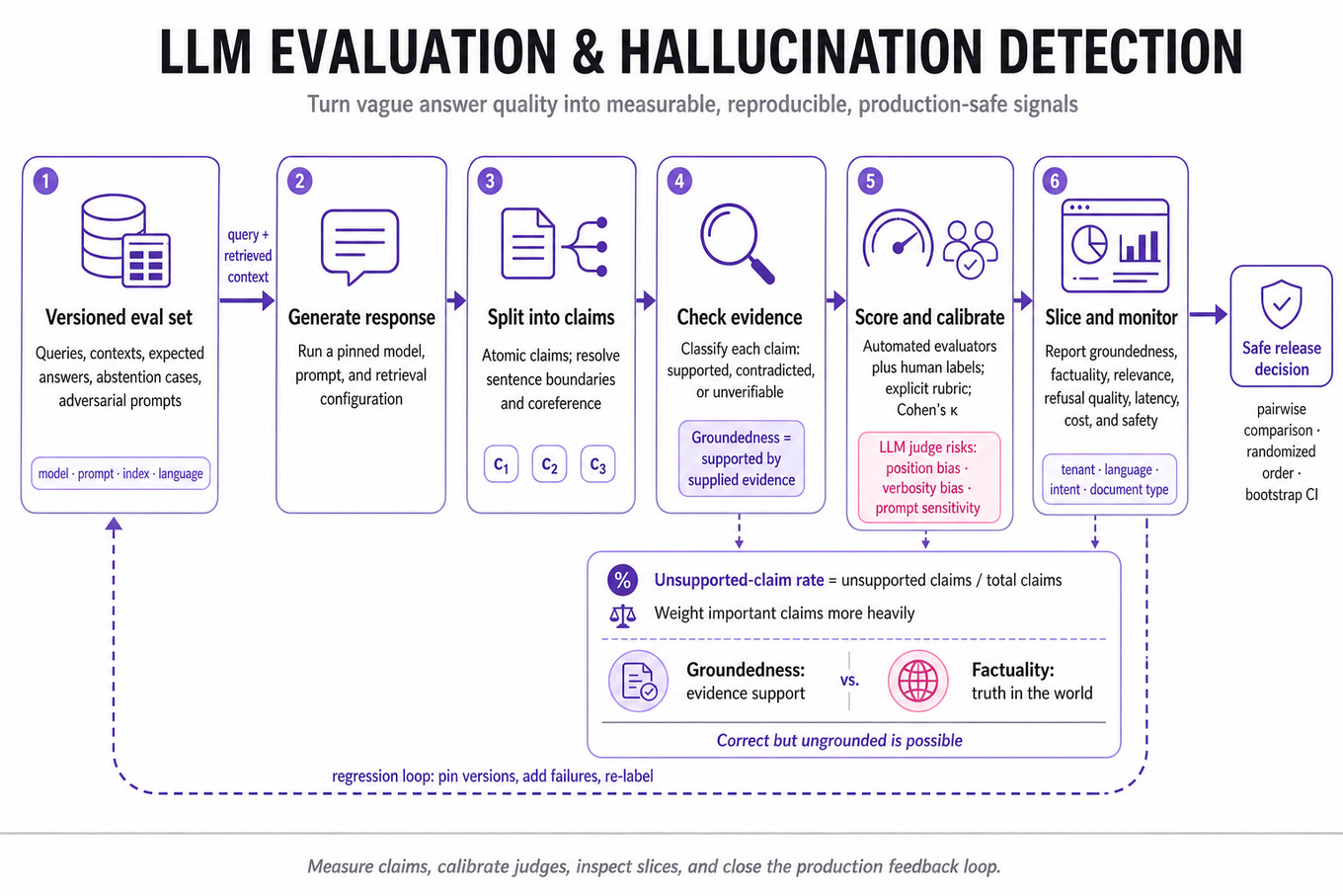
Focus area — Production LLM quality loops address your production-ML gap; focus on groundedness, hallucination checks, judge calibration, regression tests, and human review.

What's being tested

These questions test whether you can turn vague LLM quality into measurable, reproducible evaluation metrics, then build an improvement loop that operates safely in production. You must distinguish unsupported claims from stylistic variation, retrieval failures, and legitimate uncertainty, using both automated evaluators and human-labeled data. Microsoft cares because enterprise applications need dependable answers, traceable regressions, and monitoring that remains useful as prompts, models, retrieval indexes, and user traffic change.

Core knowledge

• Groundedness measures whether an answer is supported by supplied evidence, while factuality measures truth against the external world; a response can be factually correct yet ungrounded if the provided context does not support it.

• Build a versioned evaluation set containing representative queries, retrieved contexts, expected answers, abstention cases, adversarial prompts, and metadata such as domain, language, difficulty, model, prompt, and retrieval configuration.

• Use multiple metrics: citation correctness, context recall, answer relevance, groundedness, refusal quality, latency, token cost, and safety. Aggregate metrics can hide severe failures, so report slices such as tenant, language, document type, and query intent.

• For a response split into claims $c_1,\ldots,c_n$, a simple unsupported-claim rate is
  $\text{HallucinationRate}=\frac{\sum_i \mathbf{1}[\text{claim }c_i\text{ lacks support}]}{n}.$
  Weighting claims by importance is better than treating every sentence equally.

• A practical groundedness scorer splits output into atomic sentences or claims, retrieves relevant context passages, and classifies each claim as supported, contradicted, or unverifiable; sentence splitting and coreference resolution are important edge cases.

• LLM-as-a-judge scales semantic evaluation but inherits position bias, verbosity bias, model-specific blind spots, and prompt sensitivity. Calibrate it against human labels, use explicit rubrics and structured outputs, and periodically estimate agreement such as Cohen’s $\kappa$.

• Prefer pairwise comparison for prompt or model changes when absolute scoring is noisy: randomize candidate order, include ties, blind the evaluator, and bootstrap confidence intervals over query-level outcomes rather than treating each claim as independent.

• Maintain evaluation versioning: pin model versions, system prompts, retrieval settings, datasets, judge prompts, and scoring code. Otherwise, a metric change cannot be attributed to the candidate model or deployment change.

• Separate offline evaluation from production monitoring. Offline suites enable controlled regression testing; online signals include user feedback, citation clicks, correction rates, abstention rates, sampled human audits, judge scores, latency, and token consumption.

• Monitor drift across query distributions, retrieved-document distributions, embedding similarity, answer lengths, language, and failure categories. A stable average score can conceal degradation in a newly popular tenant or a low-volume safety-critical slice.

• Design the improvement loop as: collect failures, label or adjudicate them, classify root cause, modify one component, rerun the fixed regression suite, and canary the change. Root causes may be retrieval recall, chunking, prompt instructions, tool failure, model behavior, or evaluator error.

• Use risk-weighted thresholds rather than one universal gate. A minor style regression may be acceptable for a low-risk assistant, while unsupported legal, medical, financial, or administrative claims should trigger abstention, escalation, or release blocking.

Worked example: Design an Evaluation and Improvement Loop for a Production LLM Application

For “Design an Evaluation and Improvement Loop for a Production LLM Application,” I would first clarify the application’s task, grounding sources, risk tolerance, traffic, supported languages, latency budget, and whether answers must cite evidence. I would state an assumption that this is a retrieval-augmented enterprise assistant whose responses must be attributable to approved documents. I would organize the answer around four pillars: a versioned offline dataset, a layered evaluator, production monitoring with slice analysis, and a controlled deployment/improvement loop. The offline set would combine historical queries, expert-authored cases, adversarial examples, abstention cases, and sampled production traffic with human labels for groundedness, relevance, completeness, and safety. The evaluator would combine deterministic checks, retrieval diagnostics, calibrated judge models, and periodic human audits rather than relying on a single LLM score. I would explicitly trade off judge coverage and cost against human-label precision, using human review to calibrate and audit the automated evaluator. Deployment would use shadow or canary traffic, regression gates, rollback criteria, and model/prompt/retrieval version identifiers for every result. I would close by saying that, with more time, I would define an error taxonomy and test whether each intervention improves high-risk slices without merely optimizing the judge.

A second angle

For “Measure LLM Quality and Detect Hallucinations, Then Implement an Evaluation Component,” the emphasis shifts from platform lifecycle design to implementing a transparent groundedness measurement component. I would clarify whether “hallucination” means unsupported-by-context, contradicted-by-context, or globally false, because those require different labels and evidence sources. A robust implementation would extract claims, compare each claim with supplied context, return per-sentence labels and evidence spans, and aggregate with both macro and risk-weighted scores. I would call out that naive string overlap misses paraphrases and can mark a correct synthesis as unsupported, so semantic entailment or a calibrated judge is useful but must be audited. I would test empty context, multi-sentence claims, negation, pronouns, conflicting passages, and answers that appropriately abstain.

Common pitfalls

Analytical mistake: Treating an LLM judge score as ground truth is tempting, especially when it correlates with a few manually reviewed examples. A stronger answer discusses calibration against human labels, inter-rater disagreement, confidence intervals, and judge drift, while retaining deterministic and human checks for high-risk cases.

Pitfall: “The answer contains the same words as the context, so it is grounded.” Lexical overlap does not establish entailment and can miss contradictions or unsupported conclusions.

Communication mistake: Jumping directly into a specific model, vector database, or prompt template before defining quality and risk makes the design sound implementation-led. Start with the contract—what counts as a correct, supported, useful, and safely abstaining answer—then select components that measure it.

Depth mistake: Proposing only an offline benchmark misses production distribution shift and feedback loops. Explain canaries, slice-level monitoring, rollback, dataset refresh, evaluator recalibration, and root-cause attribution across retrieval, generation, tools, and data.

Connections

An interviewer may pivot to retrieval evaluation such as recall@k and nDCG, human annotation design, or experiment analysis for comparing prompts and models. They may also ask about data and concept drift, safety classifiers, abstention policies, model serving latency, and offline/online feature or configuration parity.

Further reading

• RAGAS: Automated Evaluation of Retrieval Augmented Generation — Introduces automated dimensions for faithfulness, answer relevance, and context relevance.

• FAVA: Fine-grained Atomic Verification for Factuality Evaluation — Shows why decomposing answers into atomic claims improves factuality analysis.

• TruthfulQA: Measuring How Models Mimic Human Falsehoods — A useful benchmark for understanding truthfulness failures beyond simple retrieval grounding.

Practice questions

Focus area — You selected PyTorch and will code in Python/NumPy; practice tensors, batching, losses, autograd, evaluation mode, and reproducible training loops.

What's being tested

The interviewer is testing whether you can implement, explain, and debug a complete mini-batch training loop rather than only call a high-level trainer. You should be fluent in the differences between `PyTorch` autograd and a manual `NumPy` implementation, including gradient calculation, parameter updates, batching, evaluation mode, and numerical stability. This matters for an MLE because training code must be correct, reproducible, observable, and adaptable when moving from experimentation into a production training pipeline.

Core knowledge

• A standard supervised loop has four stages: sample a batch, compute predictions and loss, compute gradients, then update parameters. For a batch $B$, empirical risk is $\hat{L}(\theta)=\frac{1}{|B|}\sum_{(x,y)\in B}\ell(f_\theta(x),y)$.

• In `PyTorch`, mark trainable tensors with requires_grad=True or use nn.Parameter; call loss.backward() to populate .grad, then update inside torch.no_grad(). The optimizer should own the update rule, such as SGD, momentum, or Adam.

• Call optimizer.zero_grad() before every backward pass unless intentionally accumulating gradients across multiple batches. Otherwise gradients add to existing values, silently changing the effective batch size and potentially causing exploding updates.

• Use model.train() during training and model.eval() during validation or inference. This changes behavior for Dropout and BatchNorm; torch.no_grad() or torch.inference_mode() prevents unnecessary graph construction but does not replace eval().

• A manual `NumPy` loop must derive gradients explicitly. For linear regression, $\hat{y}=XW+b$, residual $r=\hat{y}-y$, and mean-squared-error gradients are $\frac{\partial L}{\partial W}=\frac{2}{n}X^\top r$ and $\frac{\partial L}{\partial b}=\frac{2}{n}\sum_i r_i$.

• Preserve shape contracts. With features shaped (batch, d) and weights (d, 1), predictions should be (batch, 1); use explicit reshaping rather than accidental broadcasting. A target shaped (batch,) versus (batch,1) can produce plausible but incorrect loss tensors.

• Mini-batch sampling should shuffle training indices each epoch, cover every example once when using ordinary epoch-based SGD, and avoid shuffling validation data. drop_last=True can stabilize BatchNorm but discards examples; drop_last=False preserves data but creates a smaller final batch.

• Learning-rate behavior is often the main optimization failure. SGD updates $\theta\leftarrow\theta-\eta g$; Adam maintains first and second moments. Log loss by number of examples or batches consistently, and compare training loss with validation loss to identify overfitting.

• Use numerically stable losses. For classification, prefer torch.nn.CrossEntropyLoss, which combines log-softmax and negative log-likelihood; do not apply softmax before it. In `NumPy`, compute log-sum-exp as $z_{\max}+\log\sum_j e^{z_j-z_{\max}}$ to avoid overflow.

• Device and dtype must be consistent: move both model and batches with .to(device), and avoid repeated CPU/GPU transfers inside the inner loop. Prefer float32 for ordinary training; use mixed precision only with appropriate scaling and validation of numerical behavior.

• Validate gradients before optimizing. Compare analytical gradients with finite differences, using $\frac{L(\theta+\epsilon)-L(\theta-\epsilon)}{2\epsilon}$ for small $\epsilon$. Relative error, rather than absolute error alone, is useful when gradients vary greatly in magnitude.

• Production-quality loops checkpoint model and optimizer state, record configuration and random seeds, expose batch loss and epoch metrics, and support resume-after-failure. Save model.state_dict() plus optimizer state, epoch, scheduler state, and any scaler state used for mixed precision.

Worked example

Representative prompt: “Implement a mini-batch linear regression training loop in `PyTorch` and `NumPy`.” First, clarify the tensor shapes, loss definition, batch-size convention, stopping criterion, and whether the implementation must support GPU execution or only demonstrate the mechanics. I would organize the answer around data batching, forward and loss computation, gradient/update semantics, and validation plus instrumentation. In `PyTorch`, I would define parameters or an nn.Module, use DataLoader, call zero_grad(), compute the loss, call backward(), and invoke optimizer.step(); evaluation would use model.eval() with inference_mode(). In `NumPy`, I would compute the forward pass and analytical gradients directly, divide gradients by the actual batch size, and update weights after each batch. I would explicitly flag the tradeoff between a simple Python loop that is easy to inspect and vectorized operations that are substantially faster for large datasets. I would add assertions for shapes, finite-loss checks, and a finite-difference gradient test before trusting the loop. If I had more time, I would add checkpointing, learning-rate scheduling, deterministic seeding, and a comparison showing that both implementations converge to similar parameters.

A second angle

Representative prompt: “Debug a training loop whose loss is not decreasing.” The framing changes from implementation to diagnosis: first verify data-label alignment, target shapes, loss scaling, finite values, and whether parameters actually have nonzero gradients. Then inspect learning rate, gradient norms, accidental graph detachment, missing zero_grad(), and incorrect train()/eval() state. A strong answer distinguishes optimization failure from a data or metric bug by overfitting a tiny batch; a correct loop should drive that batch’s loss near zero for a learnable problem. The same discipline applies in both frameworks, but `NumPy` requires checking every derivative manually while `PyTorch` adds graph and device failure modes.

Common pitfalls

Analytical mistake: Saying that loss.backward() updates weights is incorrect; it only computes gradients. The optimizer performs the update, and omitting optimizer.step() leaves parameters unchanged.

Pitfall: Applying softmax before CrossEntropyLoss is a common but incorrect pattern because that loss expects unnormalized logits and performs the stable log-softmax operation internally.

Communication mistake: Listing API calls without stating invariants makes the answer hard to trust. Explain what must be true after each stage: gradients correspond to the current batch, parameters change once per intended update, and validation does not build a training graph.

Depth mistake: Blaming a plateau immediately on the learning rate misses simpler causes such as stale gradients, labels with the wrong dtype, NaNs, or an incorrect `NumPy` derivative. Start with a tiny-batch overfit test and finite-value assertions before tuning hyperparameters.

Connections

An interviewer may pivot to distributed data-parallel training, mixed-precision training, checkpoint recovery, or data and model versioning. They may also connect the loop to offline/online metric parity, experiment tracking, and training-serving skew.

Further reading

• `PyTorch` Autograd Notes — explains graph construction, gradient tracking, and evaluation contexts.

• Dive into Deep Learning, Optimization Algorithms — develops SGD, momentum, Adam, and training-loop mechanics mathematically.

• CS231n: Neural Networks Part 2 — provides practical guidance on gradient checks, initialization, and debugging optimization.

Practice questions

Focus area — You explicitly selected time-series modeling; add focused coverage on forecasting validation, leakage, seasonality, and monitoring.

What's being tested

The interviewer is testing whether you can turn a temporal prediction problem into a reliable machine learning system, not merely select an algorithm. You should be able to define the forecasting unit, horizon, granularity, available-at-prediction-time features, validation scheme, serving path, and operational metrics. Microsoft cares because forecasts often drive capacity planning, ranking, recommendations, inventory, and cloud-resource allocation; leakage, stale features, or poorly monitored models can create expensive systematic errors.

Core knowledge

• Forecasting contract: Define the entity or series, timestamp semantics, frequency, forecast horizon, prediction quantiles, retraining cadence, and latency SLA. “Predict next week” is incomplete unless you specify whether predictions are hourly, daily, per region, and generated once or continuously.

• Temporal leakage: Every feature must satisfy $t_\text{feature} \leq t_\text{prediction}$. Random train/test splits leak future behavior through rolling aggregates, normalization, backfilled labels, or revised external data; use point-in-time feature retrieval from a feature store.

• Backtesting: Use rolling-origin evaluation: train through time $t$, forecast the next horizon, advance the cutoff, and repeat. Preserve realistic gaps for label availability and feature computation; the final test window should remain untouched until model selection is complete.

• Baselines: Always compare against seasonal naive forecasts, such as $\hat{y}_{t+h}=y_{t+h-m}$ for seasonal period $m$, and simple moving-average or exponential-smoothing models. A complex model that does not beat these baselines consistently is not production-ready.

• Model families: ARIMA/SARIMA captures autoregressive, differenced, and seasonal structure; ETS models level, trend, and seasonality; tree models such as LightGBM use lag and calendar features; global neural models such as DeepAR share information across many related series.

• Feature construction: Common features include lags, rolling means and standard deviations, calendar indicators, promotions, holidays, and known-future covariates. Compute windows using only historical rows, define behavior for missing lags, and avoid using a target-derived feature whose availability differs online.

• Metrics: Use MAE for interpretable absolute error, RMSE when large misses deserve extra weight, and WAPE for aggregate business error when denominators are meaningful. For probabilistic forecasts, use pinball loss for quantiles and weighted interval score for calibrated intervals.

• Scale and aggregation: For millions of series, train a global model or cluster series rather than fitting one model per entity. Reconcile hierarchical forecasts when regional predictions must sum to a corporate total; independently accurate levels can otherwise contradict one another.

• Probabilistic output: Point forecasts hide uncertainty. Predict quantiles such as $P_{50}$, $P_{90}$, or a full distribution, then test coverage: approximately 90% of outcomes should fall below a calibrated $P_{90}$ forecast. Check both calibration and sharpness.

• Serving architecture: Batch forecasts are appropriate for daily planning; online inference is appropriate when forecasts depend on current state. Keep feature computation, model versioning, input schemas, and transformations consistent between training and serving, with fallback to a seasonal-naive model.

• Monitoring: Track data freshness, missingness, feature distributions, forecast volume, latency, error by horizon and segment, residual autocorrelation, and prediction-interval coverage. Actual-error monitoring is delayed, so use input and prediction drift as leading indicators rather than treating drift as proof of model failure.

• Operational edge cases: Handle daylight-saving transitions, timezone boundaries, series with short histories, zero-inflated or intermittent demand, new entities, outliers, delayed labels, and changed business definitions. For intermittent demand, Croston-style methods or two-stage occurrence/size models may outperform ordinary regression.

Worked example — Design a production time-series forecasting system

A strong candidate would first clarify the exact series, forecast horizon, frequency, number of entities, whether future promotions or capacity plans are known, and whether predictions are batch or online. I would state an assumption such as: “We need daily forecasts for 100,000 regional-product series, seven days ahead, refreshed each night, with $P_{50}$ and $P_{90}$ outputs.” I would organize the answer around four pillars: point-in-time data and feature generation, rolling-origin evaluation against seasonal-naive baselines, model and probabilistic-output selection, and deployment plus monitoring. I would begin with lag, rolling, calendar, and known-future features in a global LightGBM model, then compare it with a global neural model if scale and cross-series patterns justify the complexity. The explicit tradeoff is per-series models versus a global model: per-series models are easier to reason about for stable long histories, while a global model shares statistical strength and handles many short series more efficiently. I would describe a batch pipeline that materializes features, validates schemas and freshness, scores the versioned model, stores forecasts and metadata, and exposes them to downstream consumers. Evaluation would report aggregate and per-segment MAE or WAPE, horizon-specific error, quantile loss, and $P_{90}$ coverage rather than one average number. I would close by saying that, with more time, I would investigate hierarchical reconciliation, cold-start handling, backtesting under historical outages, and rollback behavior when actuals or covariates arrive late.

A second angle — Evaluate a multi-step demand forecasting model

For a question focused on evaluation, the framing changes from architecture to whether the offline result predicts production behavior. I would compare direct, recursive, and multi-output forecasting strategies because recursive error can compound across a seven-day horizon. I would use rolling backtests with the same forecast cutoffs and feature availability as production, stratify results by series volume and intermittency, and compare against seasonal-naive forecasts. I would also test interval calibration and business-weighted losses, since a model with lower average MAE may be worse when under-forecasting causes capacity shortages. Finally, I would reserve the latest time block for an untouched final check and use a shadow or canary deployment before replacing the existing model.

Common pitfalls

Pitfall: Randomly splitting rows and reporting a strong validation score is a classic leakage failure. Use chronological, rolling-origin splits and prove that every feature would have existed when the prediction was generated.

Pitfall: Saying “I would use an LSTM” without defining the target, horizon, baseline, or evaluation metric sounds like algorithm shopping. Lead with the forecasting contract and a simple deployable baseline, then justify additional complexity with measured gains.

Pitfall: Monitoring only RMSE after deployment misses stale features, broken calendars, cold-start entities, and poorly calibrated uncertainty. Describe operational checks, segment-level error, delayed-label handling, and a safe fallback path.

Connections

An interviewer may pivot to feature-store point-in-time correctness, concept drift and retraining, probabilistic calibration, or hierarchical reconciliation. They may also connect forecasting to online experimentation when predictions influence a capacity or product decision.

Further reading

• Forecasting: Principles and Practice — Hyndman and Athanasopoulos’s practical treatment of baselines, backtesting, hierarchical forecasting, and probabilistic evaluation.

• DeepAR: Probabilistic Forecasting with Autoregressive Recurrent Networks — Introduces global probabilistic forecasting across related time series.

• Temporal Fusion Transformers for Interpretable Multi-horizon Time Series Forecasting — Covers multi-horizon prediction with static, observed, and known-future covariates.

Practice questions

Analytics & Experimentation

Focus area — You selected A/B testing and viewed analytics content; emphasize experiment design, guardrails, power, ramping, and interpreting ambiguous product metrics.

What's being tested

This topic tests whether you can evaluate an ML model in production rather than relying only on offline validation. You should connect randomized experimentation, model-quality metrics, guardrails, statistical uncertainty, and operational signals such as latency and error rate. Microsoft cares because an MLE must safely determine whether a deployed model improves user-facing outcomes while preserving reliability, fairness, and online/offline consistency.

Core knowledge

• Randomized controlled experiments assign eligible units—typically users, tenants, sessions, or queries—to treatment and control using a stable hash. Randomization prevents systematic differences, but the unit must match the interference pattern: user-level assignment is safer than request-level assignment when users can receive mixed behavior.

• Treatment effect is usually estimated as $\hat{\tau}=\bar{Y}_T-\bar{Y}_C$, with a confidence interval derived from the variance of the two groups. For a ratio metric such as clicks per impression, use a principled delta-method or bootstrap approach rather than independently testing numerator and denominator.

• Primary metrics should measure the model behavior being changed: `NDCG@10`, `MRR`, recall, calibration error, or conversion rate. Define one primary success criterion before launch; otherwise repeatedly inspecting many metrics increases false-positive risk through multiple comparisons.

• Guardrail metrics detect regressions that a quality metric can hide: `p95`, `p99`, latency, timeout rate, empty-result rate, crash rate, CPU utilization, revenue-protection constraints, and complaint or abuse rates. A model that improves ranking while violating latency or safety thresholds should not ship.

• Statistical power depends on effect size, variance, traffic, and significance threshold. A rough continuous-metric approximation is $n \propto (z_{1-\alpha/2}+z_{1-\beta})^2\sigma^2/\delta^2$ per arm; detecting half the effect generally requires roughly four times the sample size.

• Sample-ratio mismatch (SRM) occurs when observed treatment/control allocation differs materially from the intended split. Investigate assignment logic, eligibility filters, exposure logging, and duplicate identities before interpreting outcomes; an SRM can invalidate otherwise impressive results.

• Exposure and intent-to-treat must be distinguished. Analyze users according to their randomized assignment for the primary estimate, even if serving fails for some requests; conditioning only on successfully exposed users can introduce post-treatment selection bias.

• Interference and contamination violate the usual independence assumption. Shared caches, collaborative recommendations, marketplace supply, or models retrained using treatment-generated data can let one arm affect another; use cluster, tenant, or geo-level randomization when individual assignment is unsafe.

• Sequential monitoring changes the false-positive rate if a team repeatedly stops when a result looks significant. Predeclare a fixed duration, use an alpha-spending or sequential-testing method, or report confidence bounds under a valid sequential framework rather than treating every peek as independent.

• Offline/online parity requires identical feature definitions, transformations, missing-value handling, model versions, and label windows. Compare feature distributions and prediction outputs between training, shadow, and production traffic; a high offline `AUC` does not compensate for serving-time feature skew.

• Heterogeneous treatment effects can reveal regressions hidden by an aggregate average: new versus returning users, language, device, geography, query class, or traffic intensity. Predefine important slices, control multiplicity, and require adequate sample sizes; post-hoc slice hunting is hypothesis generation, not proof.

• Experiment safety benefits from shadow mode, canary rollout, ramp limits, automatic rollback, and immutable model/version metadata. Keep the assignment stable across requests and preserve enough exposure, prediction, feature, and outcome information to reproduce the analysis without rebuilding the serving path.

Worked example

Evaluating a New Ranking Model with an Online A/B Test is a representative MLE scenario. In the first 30 seconds, clarify the randomization unit, eligibility rules, exposure definition, primary ranking metric, minimum detectable improvement, experiment duration, and rollback thresholds. I would organize the answer around four pillars: deterministic assignment, valid exposure and outcome logging, offline/online metric parity, and statistical analysis with operational guardrails. I would assign users to the old or new model using a stable hash, then compare `NDCG@10` or downstream qualified engagement while tracking `p99` latency, empty results, and serving failures. The main tradeoff is user-level assignment, which prevents cross-request inconsistency, versus query-level assignment, which may provide cleaner per-query comparisons but contaminates users with mixed experiences. Before trusting the result, I would check SRM, missing exposure events, feature skew, delayed labels, and whether retraining caused treatment data to leak into control. I would ship only if the primary metric clears the predeclared threshold and all guardrails remain within bounds. If I had more time, I would add preplanned segment analysis, a longer-horizon retention check, and a rollback drill.

A second angle

A related scenario is Canarying a New Feature Pipeline Before Full Experimentation, where the central risk is not only model quality but serving correctness. The model can run in shadow mode against mirrored requests, allowing comparison of predictions, feature freshness, null rates, and latency without exposing users to treatment behavior. The framing shifts from estimating causal lift to detecting parity and reliability failures before randomization. Once the canary is healthy, the same stable assignment and guardrail framework supports a causal A/B test.

Common pitfalls

Pitfall: Treating offline `AUC` or validation loss as proof of online improvement. Offline labels may be biased, stale, or disconnected from the serving objective; connect the metric to the deployed decision and validate it experimentally.

Pitfall: Saying “run the test until the p-value is below 0.05.” This ignores power, sequential peeking, delayed outcomes, SRM, and multiple metrics; state the stopping rule, minimum detectable effect, and guardrails before launch.

Pitfall: Focusing on statistical significance while ignoring MLE failure modes. A strong answer should explicitly cover model/version traceability, feature skew, exposure logging, latency, rollback, and what happens when the new model times out.

Connections

The interviewer may pivot to model monitoring and drift detection, feature-store and training-serving skew, canary deployment, counterfactual evaluation, or fairness across slices. Be ready to explain how experiment results feed deployment gates and how delayed or biased labels affect monitoring.

Further reading

• “Controlled Experiments on the Web: Survey and Practical Guide” — Ronny Kohavi et al.’s practical treatment of online experimentation, metrics, and common validity failures.

• “Trustworthy Online Controlled Experiments: A Practical Guide to A/B Testing” — detailed coverage of experiment design, SRM, power, guardrails, and sequential analysis.

• “The ML Test Score” — Google’s framework for testing production ML systems beyond model accuracy.

Practice questions

Software Engineering Fundamentals

Focus area — Your production gap makes API failure handling and testable Python important; emphasize contracts, retries, validation, and service boundaries.

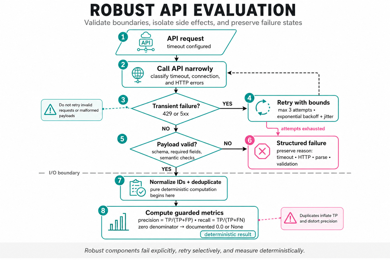
What's being tested

These questions test defensive Python programming: validating inputs, isolating side effects, handling exceptions, and producing deterministic outputs. They also probe metric correctness—especially precision/recall—and whether you can make an evaluation component robust to flaky APIs, malformed responses, retries, and partial failures.

Patterns & templates

• Separate pure computation from I/O: fetch API results first, then compute metrics or scores in deterministic, easily unit-tested functions.

• Validate at boundaries with explicit types, required fields, ranges, and allowed values; reject malformed data instead of silently coercing it.

• Wrap network calls narrowly with try/except; distinguish timeout, connection, HTTP-status, parsing, and semantic-validation failures.

• Use bounded retries with exponential backoff and jitter; retry transient 429 and 5xx responses, not invalid requests or malformed payloads.

• For top-k evaluation, deduplicate results and normalize identifiers before calculating $precision = TP/(TP+FP)$ and $recall = TP/(TP+FN)$.

• Treat zero denominators explicitly: return 0.0, None, or a documented convention rather than allowing ZeroDivisionError or misleading perfect scores.

• Represent prices as integer cents or Decimal, never binary floating point; keep validation, calculation, and presentation separate.

Common pitfalls

Pitfall: Counting duplicate API results as separate predictions inflates true positives and can make precision exceed the intended interpretation.

Pitfall: Catching broad Exception and returning an empty result hides outages; preserve an error state or structured failure reason.

Pitfall: Retrying every failure can amplify load and duplicate side effects; use timeouts, bounded attempts, and idempotency where applicable.

Practice these

The practice cards below cover the canonical variants — solve all of them and time yourself.

Practice questions