Google Data Scientist Interview Prep Guide

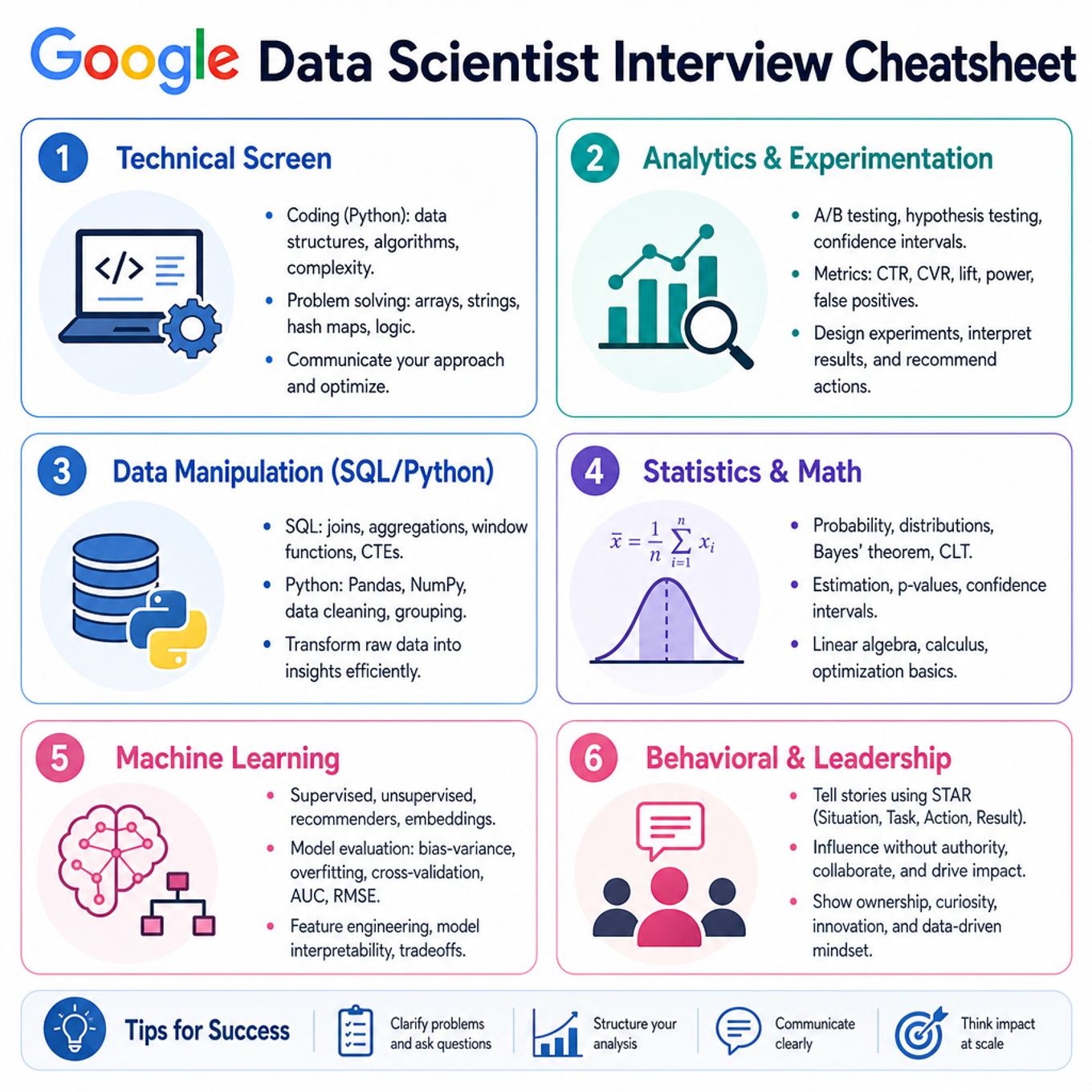
Technical Screen

Analytics & Experimentation

• A/B Testing And Product Metric Diagnostics — covered in depth under Onsite below.

• Propensity Score Matching And Observational Causal Inference — covered in depth under Onsite below.

Data Manipulation (SQL/Python)

• SQL Analytics And Event Data Manipulation — covered in depth under Take-home Project below.

What's being tested

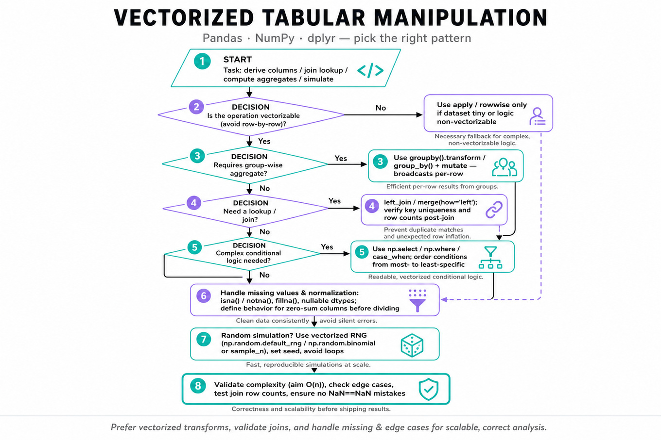
This tests vectorized tabular manipulation in pandas, NumPy, and dplyr: create derived columns, join lookup tables, compute group aggregates, and run small simulations without row-by-row loops. Interviewers are probing whether you can write correct, scalable analysis code while handling missing values, type coercion, random sampling, and edge cases.

Patterns & templates

• Vectorized conditionals — use np.select, np.where, case_when, or boolean masks; encode precedence explicitly from most-specific to least-specific condition.

• Group-wise transforms — use df.groupby(keys)[col].transform('mean') to broadcast aggregates back to rows; in dplyr, use group_by() plus mutate().

• Join then mutate — use left_join() / merge(..., how='left') to attach treatment parameters, then compute adjusted values; validate row counts after joins.

• Random simulation — use sample_n, slice_sample, np.random.binomial, or np.random.default_rng; set seeds for reproducibility and avoid repeated loops when vectorization works.

• Column normalization — compute column sums with axis=0, divide via broadcasting, and define behavior for zero-sum columns before coding.

• Missing-value semantics — NaN comparisons are false in pandas; use isna(), notna(), fillna(), and nullable dtypes deliberately.

• Complexity expectations — most solutions should be O(n) or O(n + k) time with linear memory; avoid apply(axis=1) unless data is tiny or logic is non-vectorizable.

Common pitfalls

Pitfall: Treating NaN == NaN as true or using normal comparisons on missing numeric fields; use isna() / notna() instead.

Pitfall: Creating many-to-many joins accidentally and inflating rows; check key uniqueness and compare pre/post row counts.

Pitfall: Normalizing by a zero column sum and returning inf or NaN unintentionally; specify whether to keep zeros, return NaN, or skip the column.

Practice these

The practice cards below cover the canonical variants — solve all of them and time yourself.

Practice questions

Statistics & Math

• Statistical Inference, Power, And Confidence Intervals — covered in depth under Onsite below.

• Linear Regression And OLS Inference — covered in depth under Onsite below.

Machine Learning

• Logistic Regression, Regularization, And Imbalanced Classification — covered in depth under Onsite below.

• Mixed-Effects Models — covered in depth under Onsite below.

Behavioral & Leadership

• Behavioral Leadership And Stakeholder Communication — covered in depth under Take-home Project below.

Onsite

Analytics & Experimentation

What's being tested

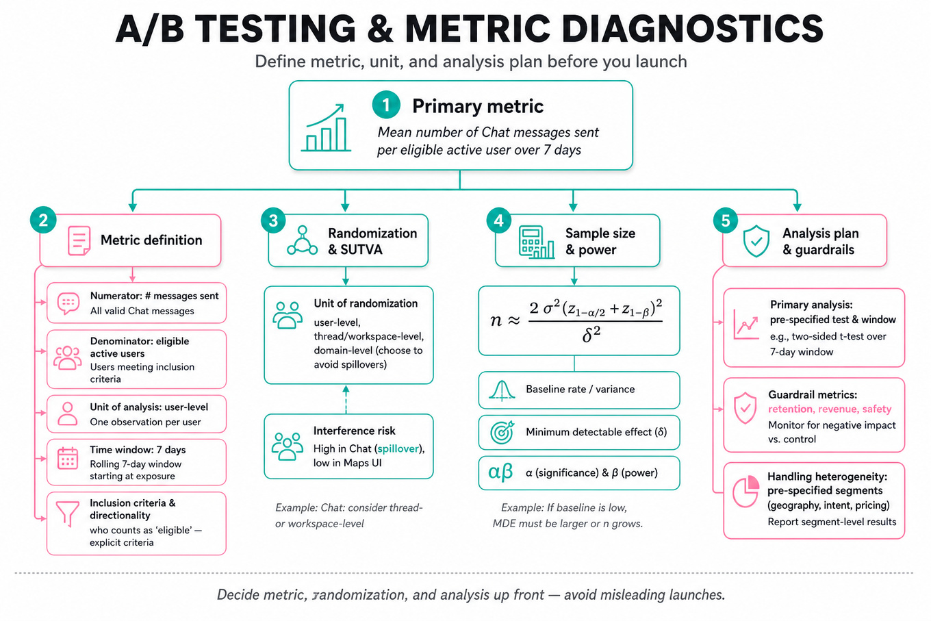
Google is testing whether you can turn an ambiguous product change into a statistically valid experiment design with a clear decision rule. Strong Data Scientist answers define the hypothesis, unit of randomization, primary metric, guardrails, sample size, segmentation, and analysis plan before talking about launch decisions. Interviewers are probing whether you understand both causal inference and product realities: network effects in Google Chat, local-intent heterogeneity in Google Maps, pricing sensitivity in subscriptions, and forecasting uncertainty in products like video views. The strongest candidates balance rigor with practicality: they know when precision matters, when speed matters, and how to avoid misleading conclusions from noisy product metrics.

Core knowledge

• Primary metric selection is the center of the design. Define numerator, denominator, unit of analysis, time window, inclusion criteria, and directionality. “Engagement increased” is weak; “mean number of Chat messages sent per eligible active user over 7 days” is interview-ready.

• Unit of randomization must match the interference structure. For UI changes in Google Maps, user-level randomization is often fine. For Google Chat, randomizing individuals can create spillovers because one treated user changes conversation behavior for untreated coworkers; consider domain-, workspace-, or thread-level assignment.

• Stable Unit Treatment Value Assumption, or SUTVA, is often violated in social and collaborative products. If treatment affects peers, the measured effect may be diluted or contaminated. Call this out explicitly for messaging, sharing, group collaboration, marketplace, and recommendation settings.

• Sample size / power depends on baseline rate, minimum detectable effect, variance, significance level, and power. For a two-sample mean comparison, a useful approximation is
  $n \approx \frac{2\sigma^2(z_{1-\alpha/2}+z_{1-\beta})^2}{\delta^2}$
  where $\delta$ is the absolute effect size you want to detect.

• Confidence level tradeoff is not automatic. 95% confidence is common, but a lower threshold may be acceptable for low-risk iteration, while higher confidence may be needed for pricing, trust, safety, or irreversible launches. Discuss false positives, false negatives, experiment duration, and opportunity cost.

• Guardrail metrics protect against local optimization. For Google Maps, guardrails might include task_success_rate, route_start_rate, latency, crash_rate, and search_refinement_rate. For pricing, use refund_rate, support_contact_rate, churn, and long-term LTV, not just immediate conversion.

• Multiple testing becomes a problem when slicing by many cohorts or tracking many outcomes. If you evaluate 20 metrics at $\alpha=0.05$, expect about one false positive by chance. Mention Bonferroni correction, Benjamini-Hochberg false discovery rate, or pre-registering primary versus secondary metrics.

• Sequential monitoring can inflate false positives if you peek daily and stop when significant. A strong answer proposes fixed analysis windows or uses methods such as alpha spending, group sequential tests, or always-valid confidence intervals. “I’ll monitor guardrails continuously but reserve success decisions for the planned readout” is a good line.

• Metric diagnostics require decomposing changes into funnel steps, cohorts, platforms, geographies, traffic sources, and user maturity. If Chat usage rises, ask whether it is more users sending messages, more messages per sender, more bots, more notifications, or a logging artifact visible in the analytical data.

• Heterogeneous treatment effects matter, but they should be framed as exploratory unless pre-specified. Pricing effects may differ by country, acquisition channel, tenure, or plan type. UI changes may help novice users and hurt power users. Avoid overfitting noisy segments into product decisions.

• Ratio metrics need careful variance handling. Metrics like messages per active user, revenue per visitor, or views per session can be analyzed with delta method, bootstrap, or user-level aggregation. Do not compare raw event-level rows if the treatment is assigned at user level; that understates uncertainty.

• Experiment validity checks are mandatory before interpreting impact. Check sample ratio mismatch, pre-period balance, exposure logging, eligibility consistency, novelty effects, seasonality, bot/internal traffic, and missingness. If assignment is 50/50, a large deviation in treatment counts is a red flag before any product conclusion.

Worked example

For Design A/B Test for Google Maps UI Change, a strong candidate starts by clarifying the product goal: is the new UI intended to improve search-to-navigation completion, reduce time to find a place, increase exploration, or improve satisfaction? They would ask who is eligible, whether the UI affects all map sessions or only certain surfaces, and whether there are safety-sensitive contexts such as driving mode. The answer can be organized around four pillars: hypothesis and population, metrics, randomization and power, and analysis / launch criteria.

A crisp setup might be: randomize eligible users at the user level, expose them consistently for two weeks, and use successful_task_completion_rate as the primary metric, defined as the share of map search sessions that lead to a meaningful action such as route start, call, website visit, or save within a fixed window. Secondary metrics could include time_to_action, search_refinement_rate, repeat_usage_7d, and user_report_rate. Guardrails should include crash_rate, latency, route_abandonment_rate, and negative feedback. One tradeoff to flag is that a broad primary metric may capture overall user value but be harder to interpret, while a narrow metric such as route_start_rate is easier to move but may miss discovery use cases. The close should be decision-oriented: launch if the primary metric improves or is neutral with strong secondary benefits, no key guardrail regresses, and effects are consistent across major platforms and regions. If more time were available, add pre-period covariate adjustment, long-term retention analysis, and qualitative review for cohorts with negative movement.

A second angle

For Design A/B Test for Subscription Price Increase Effectiveness, the same experimental logic applies, but the constraints are sharper because the intervention directly changes user cost and can affect trust. The primary metric cannot simply be conversion_rate; a higher price may lower conversion but increase revenue_per_visitor or long-term LTV. Randomization should be handled carefully across acquisition channels and geographies because users may compare prices, share screenshots, or return across devices. Guardrails should include refund_rate, chargeback_rate, support_contacts_per_signup, early churn, and brand-sensitive feedback. The tradeoff is also different: pricing tests may need longer follow-up and stronger confidence because short-term revenue lift can mask long-term retention damage.

Common pitfalls

Pitfall: Choosing a vague metric like “usage,” “engagement,” or “growth” without a precise definition.

This is the most common analytical mistake. A better answer specifies the unit, event, denominator, and window: for example, messages_sent_per_weekly_active_user among eligible Google Workspace users over 14 days, with bot-generated messages excluded or analyzed separately.

Pitfall: Treating the A/B test as only a significance test.

Interviewers expect a decision framework, not just “p-value below 0.05 means launch.” Discuss minimum detectable effect, practical significance, guardrails, confidence intervals, pre-specified readout dates, and what you would do if the result is directionally positive but underpowered.

Pitfall: Ignoring product-specific interference and heterogeneity.

For collaboration products, pricing, and local search, users are not interchangeable independent observations. Mention spillovers, cohort differences, and segment diagnostics, but avoid claiming every subgroup result is causal unless it was pre-planned or adjusted for multiple comparisons.

Connections

Interviewers may pivot from here into causal inference beyond randomized tests, such as difference-in-differences, regression discontinuity, or propensity score methods when experimentation is infeasible. They may also ask about forecasting, ranking metric evaluation, funnel diagnostics, or long-term metric design when short-term A/B results conflict with retention or user trust.

Further reading

• Trustworthy Online Controlled Experiments by Kohavi, Tang, and Xu — the standard reference for practical A/B testing, metric design, pitfalls, and organizational decision-making.

• Controlled experiments on the web: survey and practical guide, Kohavi et al. — concise coverage of online experiment design, power, ramping, and interpretation issues.

• The Seven Rules of Thumb for Web Site Experimenters, Kohavi et al. — useful heuristics for avoiding false positives, misleading metrics, and common online experimentation mistakes.

Practice questions

What's being tested

Google is probing whether you can estimate causal effects from messy product or telemetry data when a clean randomized experiment is unavailable, unsafe, or delayed. The core skill is separating correlation from causation by defining the unit of analysis, treatment, outcome, counterfactual, and likely confounders before choosing a method like propensity score matching, difference-in-differences, or controlled experimentation. Interviewers want to see that you understand both statistical identification and practical product measurement: a method is only credible if assumptions, diagnostics, and limitations are explicit. For a Data Scientist, the expected contribution is not building data pipelines, but designing the analysis, validating assumptions, interpreting uncertainty, and communicating whether the result should influence product decisions.

Core knowledge

• Propensity score matching estimates causal effects by matching treated and untreated units with similar probability of receiving treatment: $e(X)=P(T=1 \mid X)$. It is useful when treatment assignment is observational but explainable by measured covariates such as geography, device, tenure, baseline usage, or prior performance.

• The central identification assumption is conditional exchangeability: $(Y(1),Y(0)) \perp T \mid X$. In plain English, after conditioning on observed covariates, treated and control units are comparable. This fails if important unobserved factors, such as user intent or local outages, drive both treatment and outcome.

• Overlap, also called positivity, requires $0 < P(T=1 \mid X) < 1$ for relevant units. If all high-end devices get a fast experience and all low-end devices get a slow one, matching cannot estimate the effect for low-end devices under fast latency without extrapolation.

• The usual estimands are ATE, ATT, and ATC. ATE is $E[Y(1)-Y(0)]$ across everyone; ATT is $E[Y(1)-Y(0)\mid T=1]$ for treated users. Product questions often care about ATT: “what was the effect on users actually exposed?”

• A standard PSM workflow is: define pre-treatment covariates, estimate $e(X)$ with logistic regression, random forest, or XGBoost, match treated to controls, check balance, estimate the outcome difference, and compute uncertainty. The propensity model is a balancing tool, not the causal model itself.

• Balance diagnostics matter more than propensity model accuracy. Use standardized mean differences:
  $SMD=\frac{\bar X_T-\bar X_C}{\sqrt{(s_T^2+s_C^2)/2}}$
  A common target is absolute SMD < 0.1 after matching. Also inspect propensity overlap plots and covariate distributions.

• Common matching choices include nearest-neighbor matching, caliper matching, exact matching on critical variables, and stratification by propensity score bins. Calipers such as 0.2 standard deviations of the logit propensity are often used to avoid bad matches, at the cost of discarding treated units.

• Inverse probability weighting is a close alternative: weight treated units by $1/e(X)$ and controls by $1/(1-e(X))$ for ATE. For ATT, controls often receive $e(X)/(1-e(X))$. Weighting can use more data than matching but is sensitive to extreme propensities.

• Always choose covariates measured before treatment exposure. Conditioning on post-treatment variables, such as session length after latency changed or reviews written after a sales spike, can introduce collider bias or block part of the causal pathway you are trying to estimate.

• PSM is not a magic replacement for experimentation. It controls only measured confounding, can increase variance by dropping unmatched units, and may perform poorly in high-dimensional sparse settings. If randomization is feasible and ethical, an A/B test remains cleaner.

• For time-based launches, PSM alone may be insufficient because of time trends, seasonality, and simultaneous product changes. Combine matching with difference-in-differences, synthetic controls, or interrupted time-series logic when pre/post dynamics are central, as with geo usage drops or post-update call drop rates.

• Report results with uncertainty and sensitivity: confidence intervals, bootstrap standard errors, subgroup robustness, alternative calipers, and falsification checks using pre-treatment outcomes. A credible answer says, “under these assumptions, the estimated lift is X,” not “PSM proves causality.”

Worked example

For Design tests to measure latency impact, a strong candidate should first clarify the user population, the unit of analysis, and whether latency variation is randomized, naturally occurring, or caused by rollout rules. In the first 30 seconds, say: “I’d define treatment as exposure to higher page or API latency during a session, outcome as downstream engagement such as CTR, conversion_rate, watch_time, or abandonment, and I’d separate short-term session effects from user-level retention.” The answer should then organize around four pillars: measurement definition, experimental design if possible, observational causal design if randomization is not possible, and diagnostics/decision criteria.

The cleanest design is a controlled latency injection or traffic-splitting experiment, with guardrails such as p95_latency, error rate, and user harm thresholds. If intentionally slowing users is unsafe or unacceptable, use observational variation: match high-latency sessions to low-latency sessions on pre-treatment covariates like geo, device, browser, network type, time of day, prior engagement, and page type. Estimate a propensity score for receiving high latency, perform caliper matching or weighting, verify covariate balance, and compare outcomes with confidence intervals.

A key tradeoff is session-level versus user-level analysis. Session-level gives more observations but can violate independence because heavy users contribute many sessions; user-level aggregation reduces dependence but may hide acute latency effects. A strong candidate would close by saying: “If I had more time, I’d add heterogeneity analysis by device/network segment, placebo tests on pre-latency outcomes, and compare PSM estimates with difference-in-differences around known latency incidents.”

A second angle

For Establish causality: commute playlist and driving speed, the same causal logic applies, but safety and confounding dominate the framing. Treatment is listening to a commute playlist, and the outcome might be average speed, hard braking, or speeding events; the unit could be trip, driver-day, or driver. A naive comparison between playlist listeners and non-listeners is confounded by route, commute time, driver personality, traffic, weather, and baseline driving behavior. PSM could match playlist trips to non-playlist trips on pre-trip and contextual variables, but the candidate should be cautious: unobserved mood or urgency may still bias results. A randomized recommendation or encouragement design would be more credible, but any experiment must include safety guardrails and avoid inducing risky driving.

Common pitfalls

Pitfall: Treating matching as proof of causality.

A tempting answer is, “I’ll match treated and control users, compare outcomes, and conclude the treatment caused the lift.” That skips the identification assumptions. A stronger answer explicitly says PSM adjusts for observed confounders only, then checks overlap, balance, robustness, and whether unobserved confounding is plausible.

Pitfall: Matching on variables affected by the treatment.

For example, when estimating whether customer reviews affect sales, do not match on post-review traffic, ranking position after reviews changed, or conversion after reviews were visible. Those variables may be mediators or colliders. Use pre-treatment covariates such as historical sales, category, price, brand, baseline rating, seasonality, and prior traffic.

Pitfall: Overcommunicating the method and undercommunicating the decision.

Interviewers do not just want a list of causal techniques. They want to know whether the evidence is strong enough to launch, rollback, investigate, or run a follow-up experiment. Translate the estimate into product language: expected impact on DAU, revenue, retention, or safety metrics, plus uncertainty and caveats.

Connections

Interviewers may pivot from PSM to A/B testing, difference-in-differences, synthetic control, instrumental variables, or regression discontinuity depending on whether treatment was randomized, staggered, threshold-based, or naturally assigned. They may also ask about metric design, variance reduction such as CUPED, ratio metric inference, or heterogeneous treatment effects across geos, devices, and cohorts.

Further reading

• Rosenbaum and Rubin, “The Central Role of the Propensity Score in Observational Studies for Causal Effects” (1983) — the foundational paper defining propensity scores and balancing properties.

• Imbens and Rubin, Causal Inference for Statistics, Social, and Biomedical Sciences — rigorous treatment of potential outcomes, matching, weighting, and design-based causal inference.

• Austin, “An Introduction to Propensity Score Methods for Reducing the Effects of Confounding in Observational Studies” (2011) — practical overview of matching, weighting, balance diagnostics, and common mistakes.

Practice questions

Data Manipulation (SQL/Python)

• SQL Analytics And Event Data Manipulation — covered in depth under Take-home Project below.

Statistics & Math

What's being tested

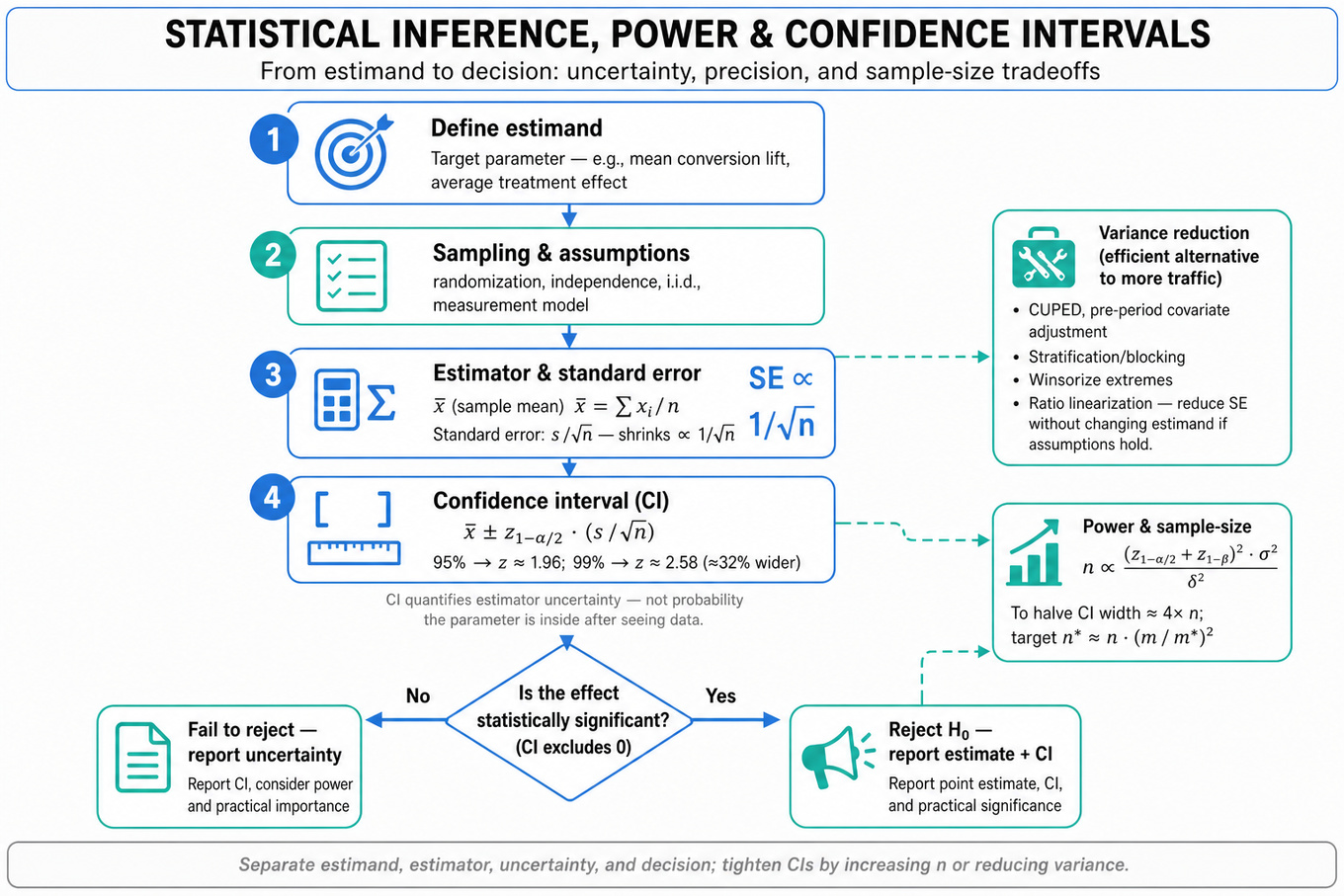
You are being tested on statistical inference as a practical decision tool: how to estimate unknown quantities, quantify uncertainty, and explain what conclusions are justified from limited data. Google Data Scientists use these skills in experiment analysis, metric monitoring, ranking evaluation, survey inference, conversion modeling, and launch decisions where noisy estimates can move product direction. Interviewers are probing whether you understand the mechanics—standard errors, confidence intervals, power, hypothesis tests, likelihoods—and whether you can communicate statistical risk without overstating certainty. Strong answers separate the estimand, sampling process, estimator, uncertainty interval, and decision rule.

Core knowledge

• Confidence intervals quantify uncertainty around an estimator, not probability that a fixed parameter lies in the interval after observation. For a sample mean, a common large-sample interval is $\bar{x} \pm z_{1-\alpha/2}\frac{s}{\sqrt{n}}$ assuming independent observations and a well-behaved sampling distribution.

• Standard error shrinks at rate $1/\sqrt{n}$, so halving a confidence interval width usually requires about $4\times$ the sample size. If the current margin of error is $m$, target margin $m^\*$ implies $n^\* \approx n(m/m^\*)^2$ when variance and confidence level stay fixed.

• Confidence level trades precision for coverage. Moving from 95% to 99% increases the critical value from about 1.96 to 2.58, widening intervals by roughly 32%. Narrowing an interval by lowering confidence is valid only if the product decision accepts greater false-certainty risk.

• Variance reduction can be more efficient than more traffic. In online experiments, techniques like CUPED, pre-period covariate adjustment, stratification, blocking, winsorization of extreme spend, and ratio-metric linearization can reduce standard error without changing the estimand if assumptions are handled carefully.

• Power is the probability of detecting a true effect under a specified alternative: $1-\beta$. For a two-sample mean test with equal groups, sample size scales roughly as $n \propto \frac{(z_{1-\alpha/2}+z_{1-\beta})^2\sigma^2}{\delta^2}$ where $\delta$ is the minimum detectable effect.

• Hypothesis tests require a null hypothesis, alternative hypothesis, test statistic, reference distribution, and decision threshold. A p-value is $P(\text{data as or more extreme} \mid H_0)$, not the probability that the null is true.

• Single-observation z-tests are only justified when the reference distribution is fully specified or its parameters are known from high-quality historical data. If $\mu$ and $\sigma$ are estimated from a small sample, use a t-test or account for parameter uncertainty.

• Percentiles from buckets require assumptions because raw ordering inside each bucket is lost. If the target rank falls within bucket $[a,b)$, linear interpolation assumes uniform density inside the bucket; without that assumption, the percentile is bounded between $a$ and $b$.

• Tail estimation is fragile. Estimating p99 latency, rare conversion, or extreme spend needs far more observations than estimating a mean, because only about 1% of samples inform p99. Bucket granularity, censoring, and top-coding can dominate statistical error.

• Maximum likelihood estimation chooses parameters maximizing $L(\theta)=\prod_i f(x_i\mid\theta)$, usually via the log-likelihood $\ell(\theta)=\sum_i \log f(x_i\mid\theta)$. MLEs are often consistent and asymptotically normal, but can be biased in finite samples, such as variance MLE using $1/n$.

• Normal conditioning is a core probability tool. If $(X,Y)$ are jointly Normal, then $Y\mid X=x$ is Normal with mean $\mu_Y+\rho\frac{\sigma_Y}{\sigma_X}(x-\mu_X)$ and variance $\sigma_Y^2(1-\rho^2).$ This underlies regression, residualization, and covariate adjustment.

• Sampling assumptions matter as much as formulas. Independence can fail with user-level clustering, repeated sessions, geo experiments, or network effects. For product metrics like CTR, conversion_rate, or revenue_per_user, define the analysis unit before computing standard errors.

Worked example

For “Narrow a confidence interval for a mean”, a strong candidate would first clarify the estimand: “Are we estimating the mean per user, per session, or per query, and is the interval for a product metric like revenue_per_user or a physical measurement?” They would ask what can be changed: sample size, confidence level, measurement method, covariates, stratification, or data quality filters. The answer should be organized around four pillars: the interval width formula, the $1/\sqrt{n}$ sample-size relationship, variance reduction, and the cost/risk tradeoff of reducing confidence.

A solid skeleton is: “For a 95% CI of a mean, width is driven by the critical value, estimated variance, and sample size. To narrow it, I can increase $n$, reduce variance, or lower the confidence level. Increasing $n$ is straightforward but costly; reducing variance through blocking, stratification, or covariate adjustment may preserve coverage while improving precision.” The candidate should explicitly flag that deleting outliers solely to shrink the interval is dangerous unless the metric definition supports winsorization or robust estimation in advance. They should also mention dependence: if observations are repeated events from the same user, the effective sample size may be closer to number of users than number of events. A good close is: “If I had more time, I’d check the empirical distribution, compute design effects from clustering, and compare a standard CI with a bootstrap or cluster-robust interval.”

A second angle

For “Estimate percentile from buckets”, the same inference mindset applies, but the constraint is information loss rather than sample-size planning. Instead of estimating a mean from raw observations, you are estimating a quantile from an aggregated histogram, so the key first step is locating the bucket containing the target rank. A strong candidate would compute cumulative counts, identify where the percentile falls, then state whether they are giving an interpolated estimate or only a bound. The tradeoff is interpretability versus assumption strength: linear interpolation is convenient, but if the distribution is skewed within the bucket, the estimate can be materially wrong. This is especially relevant for product metrics like p95 page load time or p99 serving latency, where wide upper-tail buckets can hide severe user pain.

Common pitfalls

Pitfall: Treating a confidence interval as “there is a 95% chance the true mean is inside this particular interval.”

That phrasing is tempting but not frequentist. A better explanation is: “If we repeated this sampling process many times and built intervals the same way, about 95% would contain the true parameter.” If the interviewer wants probability statements about the parameter, pivot to a Bayesian credible interval and state the prior.

Pitfall: Assuming more rows always means proportionally better precision.

For user-facing metrics, event rows may be highly correlated within users, devices, queries, or geographies. A billion pageviews from a small number of users can have less effective information than expected; use user-level aggregation, cluster-robust standard errors, or hierarchical reasoning when the analysis unit differs from the logging unit.

Pitfall: Giving formula-only answers without discussing assumptions.

Interviewers often care less about memorizing $z\sigma/\sqrt{n}$ than about knowing when it fails. Mention skew, heavy tails, small samples, estimated variance, selection bias, missingness, and non-random sampling. A practical Data Scientist should say what they would check before trusting the interval or p-value.

Connections

Interviewers may pivot from this topic into A/B testing, multiple comparisons, Bayesian inference, causal inference, or metric design. The same ideas also show up in ranking evaluation, where offline metrics like NDCG, CTR, and long_click_rate need uncertainty estimates before comparing model variants.

Further reading

• Casella and Berger, Statistical Inference — rigorous treatment of estimators, likelihood, confidence intervals, and hypothesis testing.

• Kohavi, Tang, and Xu, Trustworthy Online Controlled Experiments — practical experimentation guidance for product Data Scientists, including power, variance, metrics, and pitfalls.

• Deng et al., “Improving the Sensitivity of Online Controlled Experiments by Utilizing Pre-Experiment Data” — introduces CUPED, a widely used variance-reduction method for online experiments.

Practice questions

What's being tested

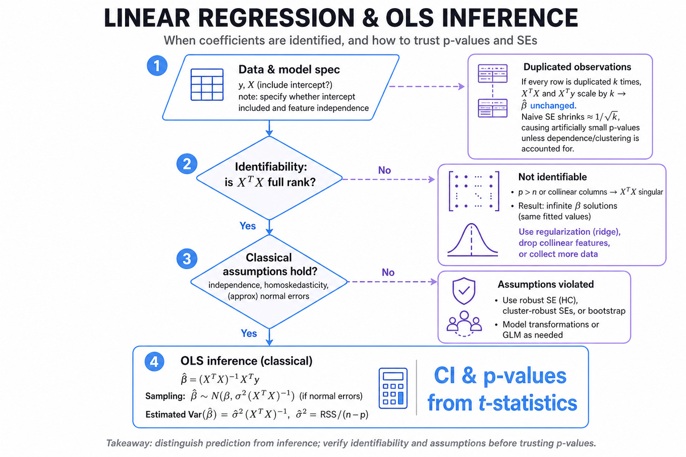
Interviewers are probing whether you understand ordinary least squares beyond fitting `LinearRegression()` and reading a coefficient table. You need to reason from first principles about identifiability, sampling variance, standard errors, p-values, feature transformations, and what changes when data assumptions are violated. Google cares because Data Scientists often use regression for metric decomposition, experiment analysis, pricing or ads diagnostics, and causal-ish adjustment; wrong inference can turn a duplicated log row or high-dimensional feature set into a false product conclusion. Strong answers separate prediction from inference, effect size from statistical significance, and algebraic invariance from modeling choices like regularization.

Core knowledge

• OLS objective estimates coefficients by minimizing squared residuals:
  $\hat\beta = \arg\min_\beta \|y - X\beta\|_2^2.$
  If $X$ has full column rank, $\hat\beta = (X^\top X)^{-1}X^\top y.$ For DS interviews, always state whether an intercept is included and whether features are linearly independent.

• Identifiability requires enough independent information to estimate parameters. If $p > n$ or columns of $X$ are collinear, $X^\top X$ is singular and infinitely many $\beta$ vectors can produce the same fitted values. You can still predict with constraints, but plain OLS coefficients are not uniquely identified.

• Sampling distribution under classical assumptions is
  $\hat\beta \sim N\left(\beta, \sigma^2(X^\top X)^{-1}\right)$
  if errors are normal, or approximately normal by large-sample arguments. The estimated variance is $\widehat{\mathrm{Var}}(\hat\beta)=\hat\sigma^2(X^\top X)^{-1}, \quad \hat\sigma^2=\frac{\mathrm{RSS}}{n-p}.$

• Duplicated observations do not create new independent evidence. If every row is duplicated $k$ times, $\hat\beta$ is unchanged because both $X^\top X$ and $X^\top y$ are multiplied by $k$. Naive standard errors shrink roughly by $1/\sqrt{k}$, causing artificially smaller p-values unless dependence or clustering is accounted for.

• P-values measure compatibility with a null effect, not practical importance. With very large $n$, tiny effects can be statistically significant; with small or noisy samples, meaningful effects may be non-significant. In product settings, pair p-values with confidence intervals, business impact, and metrics like lift in `CTR`, retention, or revenue.

• Effect-size metrics such as $R^2$, adjusted $R^2$, RMSE, MAE, and coefficient magnitude answer different questions. $R^2$ can remain unchanged under duplicated rows even as p-values become tiny. For skewed or imbalanced outcomes, MAE, quantile loss, calibration by segment, or weighted metrics may communicate model quality better than aggregate RMSE.

• Invertible linear transformations of features preserve fitted values for unregularized OLS. If $Z = XA$ for invertible matrix $A$, then coefficients transform as $\hat\gamma = A^{-1}\hat\beta$, and predictions satisfy $Z\hat\gamma = X\hat\beta$. Coefficients change coordinate systems; predictions remain the same.

• Regularization breaks some invariances because penalties depend on the coordinate representation. Ridge regression minimizes $\|y-X\beta\|^2+\lambda\|\beta\|_2^2$ and is sensitive to feature scaling, though it is rotationally more stable than lasso. Lasso minimizes $\|y-X\beta\|^2+\lambda\|\beta\|_1$ and can select different variables under correlated or transformed features.

• High-dimensional regression needs constraints or assumptions. When $p > n$, use ridge for stable prediction, lasso or elastic net for sparse signals, dimensionality reduction such as PCA, or domain-driven feature grouping. For inference after variable selection, naive p-values are invalid unless using methods designed for post-selection inference or sample splitting.

• Robust inference matters when assumptions fail. Heteroskedasticity invalidates classical standard errors even if coefficients remain unbiased under exogeneity; use heteroskedasticity-robust standard errors like Huber-White sandwich estimators. Repeated users, sessions, or geo units often require cluster-robust standard errors at the independent assignment or sampling unit.

• Communication is part of the skill. To non-technical stakeholders, describe regression as estimating the average relationship between inputs and an outcome while holding included variables fixed. Avoid saying “X causes Y” unless the design supports causality through randomization, quasi-experiment design, or a credible identification strategy.

• Diagnostics should be tied to the decision. Residual plots, leverage and influence checks, multicollinearity via VIF, train/test error, and segment-level performance reveal different failure modes. For Google-scale product data, the issue is often not computational feasibility but whether billions of rows represent independent units or repeated measurements.

Worked example

For Analyze Linear Regression Changes with Duplicated Observations, a strong candidate would first clarify whether rows are duplicated exactly, whether all rows or only a subset are duplicated, and whether the duplicated rows represent true repeated measurements or an ETL/logging artifact. They would state an assumption: “If every observation is duplicated identically and treated as independent by the model, the point estimate stays the same, but naive inference changes.”

The answer skeleton should have four pillars. First, show the algebra: duplicating all data $k$ times multiplies $X^\top X$ and $X^\top y$ by $k$, so $\hat\beta$ is unchanged. Second, explain that RSS also multiplies by $k$, but the apparent sample size increases, so standard errors usually shrink and t-statistics inflate. Third, distinguish valid repeated evidence from artificial duplication: if these are not independent draws, smaller p-values are misleading. Fourth, discuss practical implications: $R^2$ and fitted values may stay the same while p-values and confidence intervals become overconfident.

A good tradeoff to flag is whether to deduplicate the data or use weights/cluster-robust standard errors. If duplication is a logging artifact, deduplication is the cleanest analysis choice; if rows reflect repeated observations from the same user or item, the right unit of independence may be user-level clustering or aggregation. The close could be: “If I had more time, I would inspect duplication patterns by user, timestamp, and feature vector, then rerun the model with deduplicated data and cluster-robust inference to quantify how much the conclusion depends on independence assumptions.”

A second angle

For Estimate b when features exceed samples, the same core idea shifts from duplicated information to insufficient independent information. Instead of $X^\top X$ becoming artificially large through repeated rows, it becomes non-invertible because there are more parameters than independent constraints. The candidate should say that OLS coefficients are not uniquely estimable, even though many coefficient vectors may fit the training data perfectly. The practical response is to introduce structure: ridge for stable prediction, lasso if sparsity is plausible, PCA if signal lies in a lower-dimensional subspace, or collect more data if interpretability of individual coefficients is required. The interviewer may then push on inference, where the key point is that standard OLS p-values do not automatically apply after regularization or feature selection.

Common pitfalls

Pitfall: Saying duplicated observations “improve accuracy because sample size increases.”

This is the classic analytical mistake. Exact duplicates do not add independent information; they only make software believe the evidence is stronger. A better answer separates point estimates, standard errors, p-values, and effect sizes.

Pitfall: Explaining regression only as “drawing the best-fit line.”

That communication may work for one feature, but it hides the “holding other variables fixed” interpretation and fails for high-dimensional product data. For non-technical stakeholders, say regression estimates an average relationship between inputs and an outcome, then immediately caveat that association is not causation unless the data design supports it.

Pitfall: Treating regularization as a minor implementation detail.

Ridge and lasso change the estimator, the interpretation, and the inference story. In high-dimensional settings, they are not just ways to “make inverse work”; they encode assumptions about coefficient size or sparsity and can change which features appear important.

Connections

Interviewers can pivot from here to causal inference, especially omitted-variable bias, randomized experiments, and regression adjustment. They may also move into model evaluation for regression, including RMSE versus MAE, calibration, segment-level residual analysis, and robustness under skewed outcomes. Adjacent statistics topics include multicollinearity, heteroskedasticity-robust inference, bootstrap confidence intervals, and multiple hypothesis testing.

Further reading

• Hastie, Tibshirani, and Friedman, The Elements of Statistical Learning — strong treatment of OLS, ridge, lasso, and high-dimensional prediction.

• Angrist and Pischke, Mostly Harmless Econometrics — practical framing for regression inference, standard errors, and causal interpretation.

• Wasserman, All of Statistics — concise reference for sampling distributions, confidence intervals, and hypothesis testing.

Practice questions

Machine Learning

What's being tested

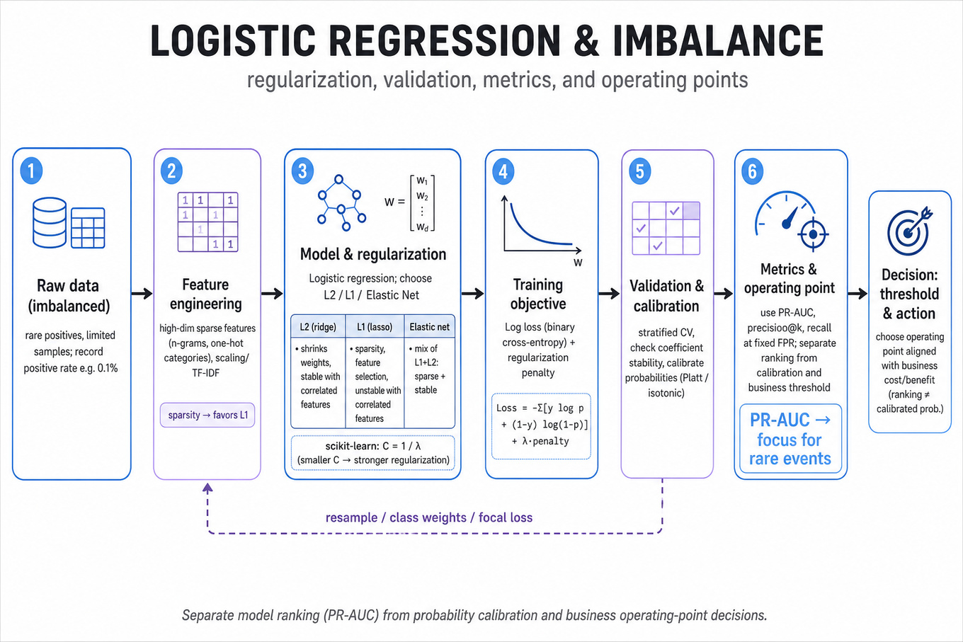
Interviewers are probing whether you can choose, diagnose, and evaluate a binary classification model under realistic data constraints: limited samples, high-dimensional sparse features, overfitting risk, and severe class imbalance. For a Data Scientist at Google, this matters because many product problems are rare-event predictions: spam, abuse, churn, conversion, fraud-like behavior, or low-frequency user actions. The expected answer is not “use logistic regression” or “use random forest,” but a structured explanation of model assumptions, regularization, validation design, metric choice, and thresholding. Strong candidates also separate model quality from business decision quality: ranking users well, calibrating probabilities, and choosing an operating point are related but distinct tasks.

Core knowledge

• Logistic regression models the conditional probability of a binary label as
  $P(y=1 \mid x)=\sigma(w^\top x+b)=\frac{1}{1+e^{-(w^\top x+b)}}.$
  It is linear in the log-odds: $\log \frac{p}{1-p}=w^\top x+b$, making coefficients relatively interpretable when features are well-defined.

• Log loss, or binary cross-entropy, is the standard training objective:
  $-\sum_i \left[y_i\log(p_i)+(1-y_i)\log(1-p_i)\right].$
  It rewards calibrated probabilities more than simple accuracy. In rare-event problems, small probability errors on many negatives can dominate the objective.

• L2 regularization adds $\lambda \lVert w\rVert_2^2$ to the loss, shrinking coefficients smoothly toward zero. It helps when features are correlated or when there are many weak predictors. In scikit-learn, smaller C means stronger regularization because C = 1 / lambda.

• L1 regularization adds $\lambda \lVert w\rVert_1$, which can set coefficients exactly to zero. This is useful for high-dimensional sparse data, such as one-hot encoded categories or text n-grams, where feature selection and interpretability matter. It can be unstable with highly correlated features.

• Elastic net combines L1 and L2 penalties: $\lambda(\alpha \lVert w\rVert_1 + (1-\alpha)\lVert w\rVert_2^2)$. It is a good answer when you want sparsity but also want more stable behavior across correlated predictors than pure L1 provides.

• Overfitting in logistic regression appears as high training performance but much lower validation performance, large coefficient magnitudes, unstable coefficients across folds, or performance that collapses on newer cohorts. Remedies include stronger regularization, fewer features, better feature grouping, cross-validation, and leakage checks.

• Underfitting appears when both train and validation performance are poor. Causes include missing nonlinearities, overly strong regularization, weak features, or an inappropriate linear decision boundary. Adding interaction terms, monotonic transformations, splines, or trying tree-based models can help.

• Random Forest models nonlinear interactions and feature thresholds automatically, but with limited data it may overfit, produce less stable probability estimates, and be harder to interpret. Logistic regression often wins when $n$ is small, features are sparse/high-dimensional, and the signal is approximately additive in log-odds.

• Class imbalance makes raw accuracy misleading. If positives are 1%, a classifier predicting all negatives gets 99% accuracy but zero recall. Start by preserving prevalence in validation/test splits using stratified sampling, then evaluate metrics aligned with the use case.

• AUROC measures ranking quality: the probability that a randomly chosen positive receives a higher score than a randomly chosen negative. It is threshold-independent and robust for comparing rankers, but it can look deceptively high when positives are extremely rare because false positives may be diluted among many negatives.

• Precision-recall AUC is often more informative for rare-event detection because it focuses on positive-class retrieval. Use precision, recall, F1, PR-AUC, and recall-at-fixed-precision when the product cost is dominated by false positives or limited review capacity.

• Threshold selection is a decision problem, not just a modeling problem. Choose a threshold using validation data based on cost: maximize expected utility, satisfy precision $\geq 95\%$, hit recall targets, or fit a human-review budget. Never pick the threshold on the test set.

Tip: A strong DS answer usually separates four layers: data split and leakage prevention, model choice, metric choice, and threshold/business decision.

Worked example

For Build Classifier: Evaluate with AUROC for Imbalanced Data, a strong candidate would first clarify the base rate, the cost of false positives versus false negatives, whether the model is used for ranking or automated action, and whether labels are delayed or noisy. They might state an assumption like: “I’ll assume positives are rare, around 1%, and the product wants to prioritize likely positives for review or intervention.” The answer should be organized around four pillars: create a leakage-safe stratified train/validation/test split, train a simple regularized baseline such as logistic regression, evaluate ranking quality with AUROC and PR-AUC, then choose a threshold using validation-set precision/recall tradeoffs. They should explain that AUROC is useful because it is threshold-independent and measures rank ordering, but it may not fully capture operational performance under extreme imbalance. A good candidate would add a calibration check using reliability curves or Brier score if downstream users interpret scores as probabilities. For imbalance mitigation, they could mention class weights, downsampling negatives, or focal loss-style approaches, while noting that resampling changes the training distribution and may require calibration afterward. One explicit tradeoff to flag is that optimizing recall may flood the product with false positives, while optimizing precision may miss many true positives. They can close with: “If I had more time, I would compare a regularized logistic baseline against a tree-based model, validate across cohorts or time splits, and run sensitivity analysis across thresholds.”

A second angle

For Compare Logistic Regression and Random Forest in Limited Data Scenarios, the same concepts appear through model selection rather than metric selection. With limited data, a regularized logistic model can have lower variance, clearer coefficients, and more stable out-of-sample performance than a RandomForestClassifier. A Random Forest may still be attractive if the signal depends on nonlinear feature interactions, but the candidate should mention tuning tree depth, minimum samples per leaf, and validation performance to control overfitting. The framing should include interpretability: a DS may need to explain which features are associated with higher conversion, churn, or abuse risk, where logistic regression provides cleaner directional evidence. The strongest answer avoids absolutism: logistic regression is not always better with small data, but it is often the safer baseline when dimensionality is high and signal is approximately linear.

Common pitfalls

Pitfall: Using accuracy as the main metric on imbalanced data.

This is the classic analytical mistake. A model with 99% accuracy can be useless if positives are 1% of the data and it predicts every case as negative. A better answer names AUROC, PR-AUC, precision/recall at a chosen threshold, and ties the final metric to the product cost.

Pitfall: Saying “L1 prevents overfitting because it removes features” without explaining the tradeoff.

That answer is directionally true but shallow. L1 induces sparsity and can reduce variance, but it can arbitrarily choose among correlated predictors and become unstable across samples. A stronger answer compares L1, L2, and elastic net, then says how they would tune regularization strength using cross-validation.

Pitfall: Treating probability scoring and classification as the same task.

A model can rank examples well but be poorly calibrated, or be calibrated but weak at top-k retrieval. If the use case needs a prioritized queue, ranking metrics like AUROC, PR-AUC, or recall-at-k matter; if the score drives user-facing decisions, calibration and threshold-specific error rates matter.

Connections

Interviewers may pivot from here into calibration, especially reliability plots, Platt scaling, isotonic regression, and Brier score. They may also connect this topic to experiment design, asking how you would evaluate a new classifier in an A/B test, or to causal inference, asking whether model features are predictive versus actionable. Adjacent model families include GradientBoostingClassifier, XGBoost, and generalized linear models with interaction terms.

Further reading

• The Elements of Statistical Learning — Chapters on linear methods, regularization, and tree-based models give rigorous grounding.

• scikit-learn: Classification metrics — Practical definitions and implementation details for AUROC, PR-AUC, precision, recall, and calibration metrics.

• imbalanced-learn User Guide — Useful reference for resampling methods, class imbalance handling, and evaluation caveats.

Practice questions

What's being tested

Interviewers are probing whether you can recognize hierarchical data and choose a model that separates true signal from group-level noise. For a Google Data Scientist, this matters in settings like ad quality ratings, search relevance judgments, creator-level outcomes, geo experiments, and marketplace metrics, where observations are not independent. The core skill is explaining fixed effects, random effects, and partial pooling clearly enough to justify a modeling choice, interpret outputs, and avoid misleading product conclusions. You are also expected to know when a simpler regression, stratified analysis, or fully fixed-effects model is more appropriate.

Core knowledge

• Mixed-effects models combine population-level coefficients with group-specific deviations. A common linear form is $y_{ij} = X_{ij}\beta + Z_{ij}u_j + \epsilon_{ij}, \quad u_j \sim N(0, G), \quad \epsilon_{ij} \sim N(0, \sigma^2).$ Here, $\beta$ are fixed effects and $u_j$ are random effects.

• Fixed effects estimate explicit coefficients for variables whose levels are of direct interest, such as treatment assignment, device type, ad format, market, or product surface. If you need to report the effect for each specific rater, campaign, country, or experiment arm, fixed effects may be appropriate.

• Random effects model group-level variation as draws from a shared distribution. They are useful when groups are sampled from a broader population, such as raters, creators, queries, advertisers, schools, or users, and the goal is to adjust for their variability rather than estimate every group independently.

• Partial pooling is the key advantage over separate group models or dummy variables. Group estimates are shrunk toward the global mean, with more shrinkage for small-sample groups. For rater bias adjustment, a rater with 5 labels should be regularized more heavily than one with 50,000 labels.

• Random intercepts allow each group to have a different baseline: $y_{ij} = \beta_0 + \beta_1 x_{ij} + u_{0j} + \epsilon_{ij}.$ This fits cases where some raters are systematically harsh, some advertisers have consistently high quality, or some geos have higher baseline conversion.

• Random slopes allow the effect of a predictor to vary by group: $y_{ij} = \beta_0 + \beta_1 x_{ij} + u_{0j} + u_{1j}x_{ij} + \epsilon_{ij}.$ Use this when treatment effects, price sensitivity, or content-quality relationships plausibly differ across markets, raters, or segments.

• Crossed random effects handle data where observations are nested in multiple non-nested groups, such as ratings crossed by both rater and ad: $score_{ra} = \beta_0 + u_r + v_a + \epsilon_{ra}.$ This is common for human evaluation systems: each rating depends on both rater bias and item quality.

• Nested random effects handle hierarchical containment, such as users within countries, videos within channels, or students within classrooms within schools. The structure might be written as random intercepts for country/channel/video, depending on the modeling library.

• Identifiability depends on overlap. To separate rater harshness from ad quality, raters must evaluate overlapping sets of ads or be connected through a rating graph. If each rater evaluates a completely unique set of ads, rater bias and item quality are confounded.

• Estimation methods include maximum likelihood, restricted maximum likelihood or REML, and Bayesian inference. REML is often preferred for estimating variance components in linear mixed models, while maximum likelihood is useful when comparing models with different fixed effects.

• Generalized linear mixed models extend the idea to binary, count, or ordinal outcomes. For example, ad approval might use logistic mixed effects: $\text{logit}(P(y_{ij}=1)) = X_{ij}\beta + Z_{ij}u_j.$ Ratings on a 1–5 scale may require ordinal models if treating them as continuous is too crude.

• Practical scaling matters. Tools like R lme4::lmer, Python statsmodels.MixedLM, or Bayesian Stan work well for small-to-medium analyses, but very large crossed-effects problems can become expensive. At Google scale, you may prototype on samples, aggregate sufficient statistics, or use approximate hierarchical/Bayesian shrinkage rather than fitting a massive dense model naively.

Worked example

For Adjust YouTube Ad Scores Using Mixed-Effects Linear Regression, a strong candidate first clarifies the unit of observation: “Is each row a rater-ad score, and can the same ad be rated by multiple raters?” They would ask whether the score is continuous, ordinal, or binary, and whether the goal is to estimate adjusted ad quality, rater bias, or both. The natural framing is a crossed mixed model: rating score depends on fixed covariates like ad category, length, language, or policy flags, plus random intercepts for both rater and ad.

A skeleton answer could have four pillars. First, define the outcome and predictors: $score_{ra}$ as the observed score from rater $r$ on ad $a$. Second, specify a model such as $score_{ra} = \beta_0 + X_{a}\beta + u_r + v_a + \epsilon_{ra},$ where $u_r$ captures rater harshness/leniency and $v_a$ captures latent ad quality. Third, explain how partial pooling prevents overreacting to raters or ads with few observations. Fourth, describe validation: check residuals, compare adjusted scores against held-out ratings, inspect rater effects, and verify that the model improves agreement or downstream quality metrics.

A key tradeoff is whether to model ads as fixed or random effects. If the purpose is to rank a specific set of ads, ad-level effects may be the estimand; if the purpose is to adjust ratings while controlling for ad heterogeneity, random ad effects can stabilize estimates. The candidate should explicitly flag that rater-ad overlap is required; otherwise, the model cannot distinguish a harsh rater from low-quality ads. A good close would be: “If I had more time, I would test robustness with an ordinal mixed model, inspect calibration by language and region, and evaluate whether adjusted scores better predict future user-facing metrics like skips, reports, or conversions.”

A second angle

For When do you use mixed-effects models, the emphasis shifts from specifying one model to diagnosing when the modeling family is appropriate. A strong answer would say to use them when observations are correlated within groups, group-level baselines vary, and we want inference that generalizes beyond the observed groups. Examples include repeated measurements per user, ratings by human judges, geo-level experiment outcomes, and queries nested within markets. The candidate should contrast this with plain regression, which assumes independent residuals, and with fixed-effects models, which may overfit or fail to estimate effects for sparse groups. The transferable idea is still partial pooling: preserve group structure without pretending every group has unlimited data.

Common pitfalls

Pitfall: Treating random effects as “unimportant fixed effects.”

Random effects are not just a convenience for variables you do not care about. They encode an assumption that group-level deviations come from a shared distribution, enabling shrinkage and generalization. A better explanation is: fixed effects estimate specific average effects; random effects estimate variance and group deviations under a population model.

Pitfall: Ignoring the independence assumption after adding a few controls.

A tempting but weak answer is, “I’ll add rater ID as a feature in linear regression.” That may absorb bias, but it does not automatically solve correlation, sparse-group instability, or out-of-sample rater handling. A stronger answer explains why repeated ratings from the same rater violate independent-error assumptions and how a hierarchical structure addresses that.

Pitfall: Overclaiming causality from a hierarchical model.

Mixed-effects models adjust for observed and structured variation, but they do not by themselves create causal identification. If estimating a treatment effect, you still need randomized assignment, credible quasi-experimental design, or assumptions about confounding. Say clearly whether the model is for prediction, bias adjustment, variance decomposition, or causal estimation.

Connections

Interviewers may pivot from this topic to A/B testing with clustered units, variance reduction, causal inference with fixed effects, or recommender/ranking evaluation using human labels. They may also ask about robust standard errors, repeated-measures designs, or when Bayesian hierarchical models are preferable to frequentist mixed models.

Further reading

• Data Analysis Using Regression and Multilevel/Hierarchical Models, Gelman and Hill — Practical treatment of hierarchical modeling, partial pooling, and applied interpretation.

• Fitting Linear Mixed-Effects Models Using lme4, Bates et al. — Seminal reference for lme4, model specification, and estimation details.

• Regression and Other Stories, Gelman, Hill, and Vehtari — Modern applied regression perspective with clear discussion of modeling assumptions and uncertainty.

Practice questions

Behavioral & Leadership

• Behavioral Leadership And Stakeholder Communication — covered in depth under Take-home Project below.

Take-home Project

Data Manipulation (SQL/Python)

What's being tested

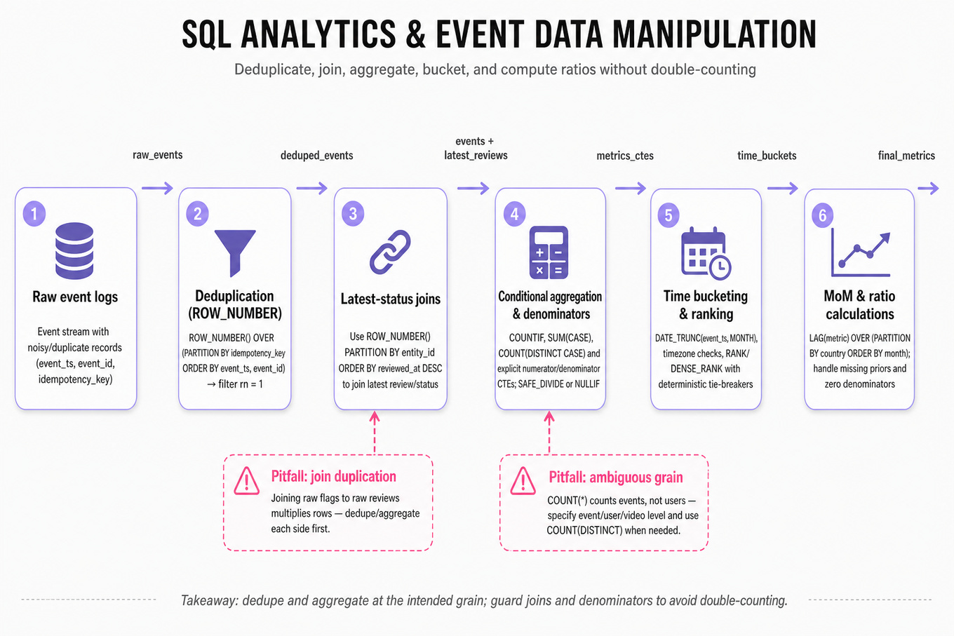
These problems test analytical SQL over event-level product data: deduplicating noisy logs, joining event and review tables, defining metric denominators, and computing time-windowed aggregates. Interviewers are checking whether you can turn ambiguous product questions into correct GROUP BY, window-function, and conditional-aggregation logic without double-counting users, flags, videos, or events.

Patterns & templates

• Deduplication with ROW_NUMBER() OVER (PARTITION BY idempotency_key ORDER BY event_ts, event_id); filter rn = 1 before aggregating.

• Latest-status joins use ROW_NUMBER() OVER (PARTITION BY entity_id ORDER BY reviewed_at DESC) to avoid many-to-one review duplication.

• Conditional aggregation with COUNTIF(...), SUM(CASE WHEN ... THEN 1 ELSE 0 END), and COUNT(DISTINCT CASE WHEN ... THEN user_id END).

• Metric ratios require explicit numerator and denominator CTEs; use SAFE_DIVIDE, NULLIF, or COALESCE for zero-denominator cases.

• Time bucketing with DATE_TRUNC(event_ts, MONTH) or DATE(event_ts); confirm timezone, inclusive/exclusive bounds, and event timestamp source.

• Ranking with RANK, DENSE_RANK, or ROW_NUMBER; specify tie behavior and deterministic secondary ordering like ORDER BY cnt DESC, product_id.

• MoM change with LAG(metric) OVER (PARTITION BY country ORDER BY month) and formula (curr - prev) / prev; handle missing prior months.

Common pitfalls

Pitfall: Joining raw flags to raw reviews can multiply rows; aggregate or deduplicate each side to the intended grain before joining.

Pitfall: COUNT(*) usually counts events, not users or entities; state whether the metric is event-level, user-level, video-level, or country-month-level.

Pitfall: Filtering after a LEFT JOIN in the WHERE clause can accidentally turn it into an INNER JOIN; put review-status filters in ON or conditional aggregates.

Practice these

The practice cards below cover the canonical variants — solve all of them and time yourself.

Practice questions

Behavioral & Leadership

What's being tested

Interviewers are probing whether you can turn data science work into organizational decisions, not just produce technically correct analysis. For a Data Scientist at Google, this means aligning product, engineering, UX, research, legal, and leadership around metric definitions, experimental evidence, modeling tradeoffs, and uncertainty. Strong answers show you can influence without authority: clarify the decision, quantify tradeoffs, communicate confidence and risk, handle pushback, and drive a measurable outcome. The best responses combine behavioral structure with DS-specific depth: experiment design, causal reasoning, metric interpretation, segmentation, and model evaluation.

Core knowledge

• STAR-L structure is the safest behavioral scaffold: Situation, Task, Action, Result, Learning. For senior DS answers, the “Action” should include analytical choices, stakeholder communication, tradeoff framing, and decision impact—not just “I built a model” or “I made a dashboard.”

• Decision-first framing beats analysis-first storytelling. Start by naming the decision: launch or rollback, change ranking objective, reallocate traffic, redefine North Star metric, or prioritize a cohort. Then explain what evidence was needed, what uncertainty remained, and how stakeholders used your recommendation.

• Stakeholder mapping matters because DS recommendations often affect teams differently. Product may optimize DAU, engineering may worry about latency, sales may care about enterprise adoption, and policy may care about fairness. A strong candidate explicitly identifies incentives, constraints, and non-negotiables before presenting results.

• Metric hierarchy helps resolve debates. Separate the primary metric such as revenue_per_user, search_success_rate, or watch_time from guardrail metrics such as latency, crash_rate, unsubscribe_rate, or complaint_rate. When metrics conflict, quantify the frontier: “+1.8% engagement, -0.4% retention, no statistically detectable change in complaints.”

• Experiment interpretation should include effect size, uncertainty, and business relevance. Use confidence intervals or Bayesian credible intervals, not only p-values: $\hat{\tau} = \bar{Y}_{treatment} - \bar{Y}_{control}$ with a 95% CI. A “significant” +0.05% lift may be irrelevant if rollout cost or risk is high.

• Causal inference discipline is essential when randomized experiments are unavailable. Mention difference-in-differences, propensity score matching, synthetic controls, or instrumental variables only when assumptions fit. For example, diff-in-diff requires parallel pre-trends; matching cannot fix unobserved confounding.

• Segmentation and heterogeneity are often where persuasion happens. Overall lift can hide harm to key cohorts via Simpson’s paradox. Break down by geography, device type, tenure, acquisition channel, model confidence bucket, or creator/viewer side of a marketplace, but control false discovery using approaches like Benjamini-Hochberg when many slices are tested.

• Model evaluation tradeoffs should be communicated in product language. Instead of saying “AUC improved from 0.81 to 0.84,” translate impact: better ranking quality, fewer false positives, improved calibration, or reduced manual review burden. For classification, discuss precision/recall tradeoffs; for ranking, use NDCG, MAP, or long-term engagement guardrails.

• Ambiguity leadership means making progress when data is incomplete. Good answers show you decomposed ambiguity into testable hypotheses, triangulated evidence from logs, experiments, surveys, and qualitative feedback, and proposed reversible decisions when confidence was moderate. Avoid pretending the data gave certainty it did not have.

• Executive communication should separate headline, evidence, recommendation, and caveats. A useful format is: “Recommendation: launch to 25% traffic. Evidence: +2.3% CTR, neutral retention, slight +0.2% latency. Risk: possible creator-side dissatisfaction in small markets. Mitigation: staged rollout and cohort monitoring.”

• Conflict handling should be specific and respectful. Strong candidates describe pushback as a signal to refine assumptions, not as a personal obstacle. They might run a pre-read, align on metric definitions, show sensitivity analyses, or propose a decision rule before results are known to reduce post-hoc debate.

• Measurable impact needs both analytical and organizational outcomes. Examples: reduced decision cycle from 4 weeks to 1 week, prevented a risky launch, improved conversion_rate by 3%, reduced false positive rate by 15%, or established a metric framework adopted by three product teams.

Worked example

For “Demonstrate stakeholder communication and influence,” a strong candidate would frame the first 30 seconds around the decision, the audience, and the conflict: “I’ll describe a case where product wanted to launch a recommendation change because offline NDCG improved, but my analysis showed mixed online effects and risk to a high-value cohort.” Clarifying assumptions should include who the stakeholders were, what decision was at stake, what metrics mattered, and whether there was an experiment or observational analysis.

The answer skeleton should have four pillars. First, define the decision and stakeholder incentives: product wanted growth, engineering wanted a simple launch path, and leadership wanted confidence in user impact. Second, explain the DS work: metric audit, experiment readout, cohort analysis, and uncertainty quantification. Third, describe communication: pre-read with product, simplified metric narrative for executives, and a tradeoff table comparing full launch, staged launch, and no launch. Fourth, close with outcome: the team chose a staged rollout, monitored guardrails, and achieved measurable lift without harming retention.

A specific tradeoff to flag: offline model quality and online product impact can diverge. For example, the model may improve NDCG@10 but over-rank popular content, increasing short-term clicks while reducing creator diversity or long-term satisfaction. A strong candidate would say they recommended a 10% traffic ramp with pre-specified decision rules: launch if CTR improved by at least 1%, 7_day_retention was non-negative within the confidence interval, and complaints did not increase.

The close should include reflection: “If I had more time, I would have designed a longer holdout to estimate retention and creator ecosystem effects, but given launch pressure, the staged rollout balanced learning speed and user risk.”

A second angle

For “Demonstrate leadership in data ambiguity,” the same underlying skill appears under less certainty and more diagnostic pressure. Instead of persuading stakeholders after a clean analysis, you may need to lead when a metric drops, an experiment is underpowered, or data sources disagree. The framing should emphasize hypothesis generation: instrumentation change, seasonality, product mix shift, ranking model drift, or true user behavior change. The communication challenge is to prevent premature conclusions while still recommending action, such as pausing rollout, expanding analysis by cohort, or running a targeted follow-up experiment. The strongest answer shows calm prioritization: “Here is what we know, what we do not know, what we can rule out today, and what decision I recommend given the cost of being wrong.”

Common pitfalls

Pitfall: Treating the story as generic teamwork instead of Data Science leadership.

Saying “I scheduled meetings, listened to concerns, and got alignment” is too shallow. A better answer shows the analytical substance behind the influence: metric definitions, experiment validity, causal assumptions, segmentation, sensitivity analysis, and quantified tradeoffs.

Pitfall: Overclaiming certainty from imperfect evidence.

A tempting but weak answer is “the data proved my recommendation was right.” Interviewers prefer candidates who distinguish signal from uncertainty: “The experiment suggested a likely positive effect, but it was underpowered for retention, so I recommended a staged rollout with guardrails.”

Pitfall: Framing stakeholders as blockers.

Avoid language like “PM didn’t understand the data” or “engineering refused to listen.” Stronger phrasing is: “Product was optimizing for launch velocity, while I was optimizing for decision quality; I reframed the discussion around user risk and decision thresholds.”

Connections

Interviewers may pivot from this topic into experiment design, metric design, causal inference, or model evaluation. Be ready to explain how you would choose a primary metric, diagnose an unexpected experiment result, evaluate a recommender system, or communicate uncertainty to non-technical leaders.

Further reading

• Thinking, Fast and Slow — useful for understanding cognitive biases that affect stakeholder interpretation of evidence.

• Trustworthy Online Controlled Experiments — practical depth on experiment design, interpretation, guardrails, and organizational decision-making.

• Google re:Work — Guide: Set goals with OKRs — helpful context for connecting DS work to measurable product and organizational outcomes.

Practice questions