Meta Data Scientist Interview Prep Guide

Technical Screen

Data Manipulation (SQL/Python)

• SQL Event Log Analytics — covered in depth under Onsite below.

Analytics & Experimentation

• A/B Testing And Experiment Design — covered in depth under Onsite below.

• Cluster Randomized Experiments And Network Interference — covered in depth under Onsite below.

• Video Calling And Group Calls Product Analytics — covered in depth under Onsite below.

What's being tested

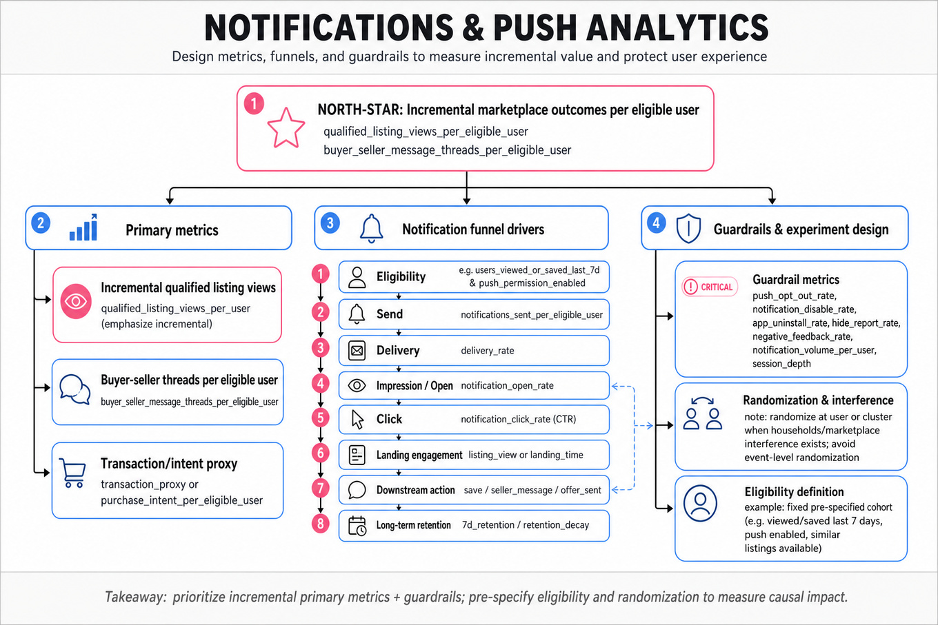
Interviewers are probing whether you can evaluate a notification product as a causal inference and measurement design problem, not just as a dashboarding exercise. Strong answers define who is eligible, what counts as exposure, what success means, and how to separate incremental value from users who were already highly engaged. Meta cares because notifications can increase marketplace liquidity, message responses, and retention, but they can also create fatigue, opt-outs, spam reports, and long-term engagement decay. The interviewer is looking for disciplined tradeoffs: growth versus user experience, short-term clicks versus durable marketplace outcomes, and individual-level effects versus network or marketplace spillovers.

Core knowledge

• Notification funnels should be decomposed into eligibility, send, delivery, impression/open, click, landing-page engagement, downstream action, and long-term retention. For marketplace, downstream metrics might include `listing_view`, `save`, `seller_message`, `offer_sent`, `purchase_intent`, or `transaction_proxy`, not just `notification_click_rate`.

• Primary metrics should reflect the product’s intended causal mechanism. For similar-listing alerts, a better primary metric than `CTR` may be incremental `qualified_listing_views_per_user` or `buyer_seller_message_threads_per_eligible_user`, because clickbait notifications can raise clicks while lowering marketplace quality or trust.

• Guardrail metrics are essential for push notifications because the treatment imposes attention costs. Common guardrails include `push_opt_out_rate`, `notification_disable_rate`, `app_uninstall_rate`, `hide_report_rate`, `negative_feedback_rate`, `session_depth`, `7d_retention`, and total notification volume per user.

• Randomization unit is usually the user for independent notification eligibility, but cluster randomization may be needed when users interact, share devices, belong to households, or participate in marketplaces with supply-demand interference. Randomizing notifications at the event level risks cross-contamination and confusing user experience.

• Eligibility definition must be fixed before analysis: for example, users who viewed or saved a marketplace item in the past 7 days, have push permissions enabled, and have at least one similar listing available. Analyze both `intent-to-treat` over eligible randomized users and treatment-on-treated for exposed users, with causal caveats.

• Power and MDE should be discussed at the user level, not notification level, because multiple sends to the same person are correlated. A basic minimum detectable effect is approximately
  $MDE \approx (z_{1-\alpha/2}+z_{power})\sqrt{\frac{2\sigma^2}{n}}$
  for equal-sized arms; clustered designs inflate variance.

• Clustered experiments require the design effect:
  $DE = 1 + (m - 1)\rho$
  where $m$ is average cluster size and $\rho$ is intracluster correlation. If households, social clusters, or geographic markets have $\rho=0.02$ and $m=50$, effective sample size drops by roughly half.

• CUPED can reduce variance using pre-experiment covariates, especially historical marketplace engagement or prior notification responsiveness. The adjusted metric is $Y' = Y - \theta(X-\bar X)$, where $\theta = \frac{Cov(Y,X)}{Var(X)}$; it helps most when pre-period and post-period behavior are highly correlated.

• Multiple testing matters when slicing by country, platform, buyer/seller role, notification type, or engagement cohort. Pre-register a primary metric and use corrections like Holm-Bonferroni or control false discovery rate with Benjamini-Hochberg for exploratory subgroup analysis.

• Heterogeneous treatment effects are often central for notifications. New users may need helpful prompts, while power users may experience fatigue. Segment by notification permission status, historical open rate, marketplace intent, inventory density, platform, and prior mute/negative feedback behavior.

• Interference and cannibalization are common. Similar-listing notifications may shift views from organic feed, search, saved items, or other notifications rather than create new demand. Measure incremental total marketplace engagement, not only engagement attributable to the new notification surface.

• Unread-rate analysis should be user-centered. For multi-account or multi-device users, compute metrics such as `unread_notifications_per_user`, `users_with_unread_rate_gt_50pct`, or bucketed account counts carefully; otherwise heavy users dominate averages and mask whether the feature worsens notification overload.

Worked example

For “How to evaluate similar-listing notifications feature,” start by clarifying the product goal: are we trying to increase buyer discovery, accelerate marketplace transactions, or re-engage users who showed shopping intent? Then define the eligible population: users who viewed or saved an item, have notification permissions, and can be matched to available similar listings within a time window. A strong answer would organize around four pillars: metric hierarchy, experiment design, segmentation, and risk monitoring. The primary metric could be `incremental_qualified_listing_views_per_eligible_user` or `buyer_seller_message_threads_per_user`, with secondary metrics like `notification_open_rate`, `save_rate`, and `return_sessions`. Guardrails should include `push_opt_out_rate`, `notification_settings_disable_rate`, `hide_report_rate`, total notifications received, and `7d_retention`.

The experiment would likely randomize at the user level: treatment users can receive similar-listing pushes, while control users continue with existing notification policy. You would analyze `ITT` first to preserve randomization, then separately inspect exposed users to understand mechanism. A key tradeoff is choosing `CTR` versus downstream marketplace actions: `CTR` is sensitive and fast, but it can reward low-quality or overly frequent notifications, so it should not be the sole success metric. You would also check cannibalization by comparing total marketplace views and messages, not just clicks from this notification. Close by saying that with more time, you would estimate heterogeneous effects by marketplace intent, notification sensitivity, and inventory density, then use those insights for targeted rollout rather than a blanket launch.

A second angle

For “Design a clustered notification experiment with guardrails,” the same evaluation logic applies, but independence assumptions become the main constraint. Instead of randomizing individual users, you may randomize clusters such as households, social graph components, geographic markets, or seller-buyer communities to reduce spillovers. The analysis must account for intracluster correlation using cluster-robust standard errors, cluster-level aggregation, or hierarchical models. The power calculation should use the design effect, because 1 million users in large correlated clusters may behave like far fewer independent observations. Guardrails become especially important because cluster-level treatment may change marketplace liquidity, seller response times, or buyer competition in ways that affect untreated users.

Common pitfalls

Pitfall: Optimizing for `notification_click_rate` alone.

This is the classic analytical mistake. A notification can produce high `CTR` by being urgent, vague, or frequent while increasing opt-outs and reducing trust. A stronger answer ties success to incremental downstream value and includes fatigue guardrails.

Pitfall: Being vague about exposure and eligibility.

Saying “compare users who got notifications to users who didn’t” is not enough, because users who receive notifications are usually more active, more permissioned, and more likely to have relevant inventory. Define the randomized eligible population first, then distinguish assignment, delivery, impression, open, and click.

Pitfall: Ignoring interference and repeated treatment.

Notifications are not one-shot independent events. Users receive many notifications, sellers may respond differently when buyer demand shifts, and one user’s action can affect another user’s marketplace experience. Call out repeated-measures correlation, cannibalization, and cluster/spillover concerns explicitly.

Connections

Interviewers may pivot from here into ranking evaluation, especially how to judge whether “similar listings” are actually relevant, or into long-term experimentation, such as novelty effects and notification fatigue. They may also ask about SQL aggregation, cohort analysis, sequential testing, or marketplace experimentation where buyer and seller outcomes must be balanced.

Further reading

• Trustworthy Online Controlled Experiments by Kohavi, Tang, and Xu — practical reference for experiment design, metrics, pitfalls, and launch decisions.

• Improving the Sensitivity of Online Controlled Experiments by Deng et al. — original CUPED-style variance reduction ideas used widely in large-scale experimentation.

• Design and Analysis of Cluster Randomization Trials by Murray — deeper treatment of intracluster correlation, design effects, and clustered experiment analysis.

Practice questions

• Ads Ranking And Monetization Analytics — covered in depth under Onsite below.

• Product Metric Design And Diagnostic Deep Dives — covered in depth under Onsite below.

Statistics & Math

• Difference-In-Differences And Staggered Rollouts — covered in depth under Onsite below.

• Statistical Inference, Power, And Metric Uncertainty — covered in depth under Onsite below.

Machine Learning

• Applied Machine Learning Modeling And Evaluation — covered in depth under Onsite below.

Behavioral & Leadership

• Cross-Functional Leadership And Analytical Communication — covered in depth under Onsite below.

Onsite

Data Manipulation (SQL/Python)

What's being tested

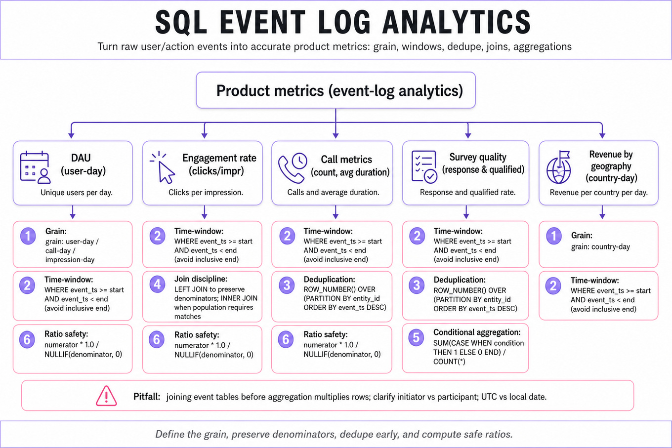
These prompts test event-log analytics: turning raw user/action tables into product metrics with correct joins, time windows, deduplication, and aggregation. Interviewers are probing whether you can write SQL that matches metric definitions precisely, especially for `DAU`, engagement rates, call duration, survey quality, and revenue by geography.

Patterns & templates

• Grain first: identify one row’s meaning before coding; aggregate to user-day, call-day, impression-day, or country-day before final metrics.

• Time-window filtering: use WHERE event_ts >= start AND event_ts < end; avoid inclusive end dates that double-count midnight events.

• Safe distinct metrics: compute COUNT(DISTINCT user_id) for users and COUNT(*) for events; never substitute one for the other.

• Join discipline: use LEFT JOIN when preserving denominators like impressions, INNER JOIN only when matched actions define the population.

• Conditional aggregation: use SUM(CASE WHEN condition THEN 1 ELSE 0 END) or COUNT_IF for clicks, responses, qualified surveys, or completed calls.

• Ratio safety: write numerator * 1.0 / NULLIF(denominator, 0); explicitly decide whether missing ratios return NULL, 0, or are filtered.

• Deduplication template: use ROW_NUMBER() OVER (PARTITION BY entity_id ORDER BY event_ts DESC) when latest valid event or one response per user is required.

Common pitfalls

Pitfall: Joining two event tables before aggregating can multiply rows, inflating clicks, responses, revenue, or duration.

Pitfall: Using the caller’s country only may miss receiver-side usage; clarify whether metrics are per initiator, participant, or call.

Pitfall: Grouping by local date when the metric requires UTC attribution changes daily trends and geography comparisons.

Practice these

The practice cards below cover the canonical variants — solve all of them and time yourself.

Practice questions

Analytics & Experimentation

What's being tested

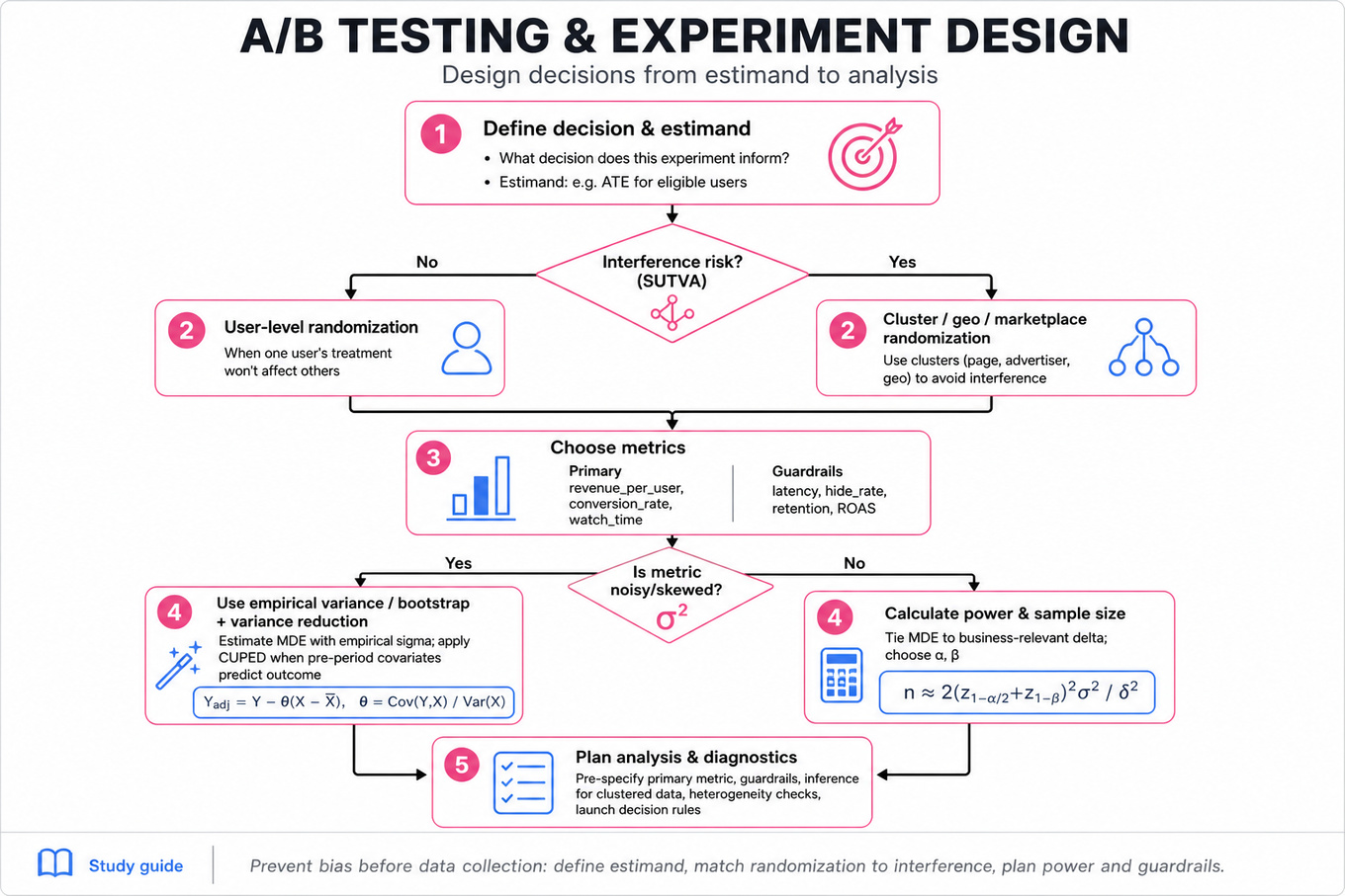
Meta Data Scientists are expected to design experiments that produce credible product and business decisions, not just compute a p-value. These prompts test whether you can define the estimand, choose the randomization unit, specify primary and guardrail metrics, reason about power, and diagnose ambiguous or null results. The interviewer is probing for practical judgment: how you handle interference in social/networked products, ads marketplace tradeoffs, noisy metrics, heterogeneous effects, and launch decisions under uncertainty. A strong answer sounds like an experiment owner who can prevent biased conclusions before data is collected and explain the result clearly after it lands.

Core knowledge

• Start with the decision and estimand: define what action the experiment informs and the causal quantity, e.g. average treatment effect $ATE = E[Y(1)-Y(0)]$ for eligible users. For ads, clarify whether the estimand is user welfare, advertiser value, platform revenue, or marketplace efficiency.

• Randomization unit must match interference risk. User-level randomization works when one user’s treatment does not affect another’s outcome. In social feeds, messaging, auctions, shops, and creator ecosystems, SUTVA may fail; consider cluster, geo, page, advertiser, or marketplace-level randomization.

• Metric hierarchy matters. Pick one primary metric such as revenue_per_user, conversion_rate, watch_time, or purchase_rate; define guardrails like hide_rate, report_rate, latency, retention, advertiser ROAS, and user experience metrics. Avoid declaring success from a post-hoc metric that moved favorably.

• Power and sample size should be tied to a minimum detectable effect. For a two-sample mean comparison with equal allocation, approximate:
  $n \approx \frac{2(z_{1-\alpha/2}+z_{1-\beta})^2\sigma^2}{\delta^2}$
  where $\delta$ is the MDE. For binary metrics, use $\sigma^2=p(1-p)$; for skewed revenue metrics, empirical variance or bootstrap estimates are more reliable.

• Variance reduction is often expected at Meta scale. CUPED adjusts outcomes using pre-experiment covariates: $Y_{adj}=Y-\theta(X-\bar X)$, where $\theta=\frac{Cov(Y,X)}{Var(X)}$. It increases sensitivity when pre-period behavior strongly predicts post-period outcomes, common for DAU, spend, engagement, and purchase metrics.

• Clustered or dependent data needs different inference. If users are randomized by cluster, effective sample size is reduced by intra-cluster correlation: $DE = 1 + (m-1)\rho$. Use cluster-robust standard errors or analyze at the cluster level; pretending millions of user rows are independent will overstate significance.

• Interference requires exposure modeling. Under network effects, define exposures such as “treated user with at least 30% treated friends” or “control user exposed to treated sellers.” You may estimate direct, indirect, and total effects, but you must state assumptions about how treatment propagates through the graph.

• Ads and ranking tests have marketplace externalities. A new shop-ads algorithm can change auction prices, advertiser budgets, organic content distribution, and user engagement. Randomizing users may measure user-side impact but miss advertiser budget reallocation; randomizing advertisers may measure advertiser value but contaminate user experience.

• Null results are not automatically failures. A null can mean no effect, underpowered design, instrumentation issues, dilution from weak exposure, heterogeneous effects canceling out, or a metric too far downstream. Check confidence intervals: “we can rule out effects larger than +0.3%” is stronger than “p > 0.05.”

• Multiple testing and peeking inflate false positives. If many segments or metrics are tested, use pre-registration, metric hierarchy, holdouts, or corrections such as Bonferroni, Benjamini-Hochberg, or alpha spending. Sequential monitoring is valid only if the stopping rule is accounted for.

• Heterogeneous treatment effects should be planned, not mined. Segment by pre-specified cohorts like new vs existing users, high vs low spenders, country, device, or advertiser size. For Meta-style products, treatment may help creators or advertisers while hurting casual users; the launch recommendation should reflect this tradeoff.

• Analysis should include diagnostics before interpretation. Check sample ratio mismatch, pre-period balance, treatment exposure, metric logging sanity, outliers, novelty effects, ramp timing, and day-of-week effects. SRM is especially serious: if assignment is 50/50 but observed traffic is 48/52, causal validity is questionable.

Worked example

For “Design an A/B test for a new shop-ads algorithm,” a strong candidate would first clarify the product change: is the algorithm changing ranking, retrieval, bidding, or targeting, and who is eligible to see shop ads? They would define the decision: launch if the new model improves marketplace value without degrading user experience or advertiser outcomes. The answer can be organized around four pillars: experiment setup, metrics, statistical analysis, and launch interpretation. For setup, they might choose user-level randomization if the main exposure is ad ranking in a user feed, but explicitly flag that advertiser budget competition creates interference, so a geo- or advertiser-level test may be needed for marketplace-level effects. For metrics, they would name a primary metric such as incremental purchase_value_per_user or ads_revenue_per_user, plus guardrails like hide_rate, report_rate, session engagement, advertiser ROAS, and small-advertiser spend concentration. For analysis, they would discuss power based on expected traffic and variance, CUPED using pre-period purchase or ad engagement, and segment checks for new shoppers, heavy shoppers, and advertiser categories. A specific tradeoff to flag: user-level randomization gives high power and clean user experience measurement, but it may underestimate budget reallocation or auction price effects. They would close by saying that, if time allowed, they would add a longer holdout or geo-level validation to capture advertiser budget dynamics and delayed purchase behavior.

A second angle

For “Design and analyze A/B test with interference,” the same experimental toolkit applies, but the core issue shifts from metric selection to causal identification. Instead of assuming each user’s outcome depends only on their own assignment, you need to model exposure through friends, groups, sellers, creators, or shared auctions. A strong answer might propose cluster randomization on graph communities, ego-network designs, or saturation experiments where clusters receive different treatment probabilities. The key difference is that the estimand may be direct effect, spillover effect, or total network effect rather than a simple user-level ATE. The analysis must use cluster-level or exposure-level inference, because independent row-level standard errors would be misleading.

Common pitfalls

Pitfall: Treating every experiment as a 50/50 user-level randomized controlled trial.

That answer is tempting because it is simple and often correct for isolated UI changes. It fails for social, ads, commerce, creator, and marketplace systems where one unit’s treatment can affect another unit’s outcome. A better answer says, “I would use user-level randomization if SUTVA is plausible; otherwise I would consider cluster, geo, advertiser, or saturation designs.”

Pitfall: Optimizing for one metric without a metric hierarchy.

Saying “launch if revenue increases significantly” is incomplete for Meta-style decisions. Ads revenue may rise while retention, hide_rate, advertiser ROAS, or content quality worsens. A stronger answer names one primary metric, a small set of guardrails, and the decision rule before looking at results.

Pitfall: Explaining a null result as “the feature does not work.”

A null result could come from insufficient power, low treatment exposure, high variance, heterogeneous effects, or delayed impact. The stronger response is to inspect confidence intervals, exposure rates, pre/post diagnostics, and planned segments, then state whether the experiment rules out a practically meaningful effect.

Connections

Interviewers may pivot from experiment design into causal inference, especially difference-in-differences, instrumental variables, or propensity methods when randomization is not possible. They may also connect this to metric design, ranking/recommender evaluation, marketplace analytics, or diagnosing anomalies in DAU, revenue, engagement, and conversion funnels.

Further reading

• Trustworthy Online Controlled Experiments — Practical industry reference on experiment design, metrics, pitfalls, and interpretation.

• Deng, Xu, Kohavi, and Walker, “Improving the Sensitivity of Online Controlled Experiments by Utilizing Pre-Experiment Data” — Seminal CUPED paper for variance reduction in online experiments.

• Kohavi, Tang, and Xu, “Seven Rules of Thumb for Web Site Experimenters” — Useful applied guidance on common online experimentation traps.

Practice questions

What's being tested

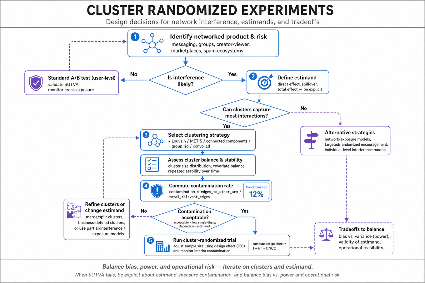
Interviewers are probing whether you can design a credible causal experiment when the standard user-level A/B test assumption breaks: one user’s treatment can affect another user’s outcomes. Meta cares because many products are inherently social—Messenger, Feed, groups, recommendations, spam enforcement, fake-account removal—and naive randomization can underestimate effects, contaminate controls, or harm user experience. A strong Data Scientist should identify network interference, define the right estimand, choose a defensible cluster randomization strategy, and explain tradeoffs in power, bias, and operational risk. The interviewer is not looking for graph-engineering implementation details; they are testing your statistical reasoning, metric design, and ability to make a launch recommendation under imperfect isolation.

Core knowledge

• SUTVA—the Stable Unit Treatment Value Assumption—requires no hidden treatment versions and no interference between units. In social products, SUTVA often fails: if Alice receives a spam-filter change, Bob’s messages_received, reply_rate, or spam_reports may change even if Bob is in control.

• Interference means a unit’s outcome depends on other units’ treatment assignments: $Y_i = Y_i(Z_i, Z_{-i})$. Common forms include direct user-to-user messaging, creator-viewer relationships, group interactions, marketplace buyer-seller effects, and adversarial ecosystems like spam or fake accounts.

• Cluster randomization assigns treatment at a group level—communities, ego networks, conversation threads, households, geographic regions, schools, or graph partitions—so most interaction edges stay within the same assignment. The goal is not perfect isolation; it is reducing cross-arm exposure enough that the estimand is interpretable.

• Graph partitioning is the usual mental model: create clusters that maximize within-cluster edges and minimize between-cluster edges, often using algorithms like Louvain community detection, METIS-style partitioning, connected components, or business-defined clusters such as group_id or conversation_id. The DS should focus on whether the resulting clusters are balanced, stable, interpretable, and low-contamination.

• Contamination rate is a key diagnostic: for a treated cluster, what fraction of relevant exposures come from control clusters, and vice versa? A simple edge-weighted version is $\text{contamination} = \frac{\sum_{(i,j): Z_i \neq Z_j} w_{ij}}{\sum_{(i,j)} w_{ij}}$ where $w_{ij}$ might be message volume, impressions, replies, or historical interaction strength.

• Estimand choice should be explicit. You may estimate the intention-to-treat effect at the cluster assignment level, the effect on highly exposed users, a spillover effect on neighbors, or a global ecosystem effect. “Average treatment effect on users” is often too vague when users have different exposure to treated peers.

• Exposure mapping translates complex networks into analyzable conditions, such as “user is treated,” “at least 50% of inbound messages come from treated senders,” or “has 2+ treated close friends.” This enables comparisons like treated-high-exposure vs control-low-exposure, but thresholds must be pre-specified to avoid fishing.

• Unit of analysis should usually match the unit of randomization or account for clustering. If randomizing by cluster but analyzing user-level rows as independent, standard errors are too small. Use cluster-level aggregation, cluster-robust standard errors, randomization inference, or hierarchical modeling depending on cluster count and metric structure.

• Power is typically worse than in user-level A/B tests because effective sample size is closer to the number of clusters than the number of users. The design effect is approximately $DE = 1 + (m - 1)\rho$ where $m$ is average cluster size and $\rho$ is intra-cluster correlation. Large clusters and high correlation can make an experiment underpowered even with millions of users.

• Cluster balance matters because social clusters can be highly skewed. You should check pre-period balance on DAU, messages_sent, spam_reports, geography, platform, tenure, and baseline outcome metrics. Use stratified or matched-pair randomization when clusters vary drastically in size or activity.

• Metric selection should separate direct product goals, guardrails, and ecosystem effects. For a Messenger spam experiment, primary metrics might include spam_message_rate, user_report_rate, message_send_success, and reply_rate; guardrails might include false_positive_rate, blocked_legitimate_messages, retention, and sender/recipient experience split by segment.

• Pre-launch analysis should quantify interference risk before the test: inspect the interaction graph, estimate cross-cluster edge share under candidate cluster definitions, simulate randomizations, compute minimum detectable effect, and identify sensitive segments. If contamination is too high, consider switchback designs, geo experiments, holdout networks, or staged rollouts.

Worked example

For “Design Messenger spam experiment with clustering”, a strong candidate would start by clarifying the treatment: “Are we changing the spam classifier threshold, sender enforcement, recipient warnings, or message delivery ranking?” They would then ask whose outcome matters—senders, recipients, conversation threads, or the broader messaging ecosystem—and declare that user-level randomization is risky because a treated sender can message a control recipient. The answer should be organized around four pillars: define the causal estimand, construct clusters from the messaging graph, choose primary and guardrail metrics, and plan inference/power under clustered assignment. For clustering, they might propose building clusters from recent high-weight messaging edges, then randomizing clusters after stratifying by size, country, and baseline spam rate. The primary estimand could be the intention-to-treat effect of enabling the new spam policy for all users in treated clusters on recipient-level spam_report_rate and legitimate message_delivery_rate. A specific tradeoff to flag is that larger graph clusters reduce cross-arm contamination but reduce the number of independent experimental units, lowering power and increasing sensitivity to outlier clusters. They should also mention analysis at the cluster level or with cluster-robust uncertainty, not naive per-message standard errors. A crisp close would be: “If I had more time, I’d run pre-period simulations to compare cluster definitions, estimate contamination, and decide whether this is feasible as an experiment or should start as a limited holdout plus observational spillover analysis.”

A second angle

For “Design experiment for fake accounts impact”, the same principles apply, but the treatment and interference path are broader. Removing or demoting suspected fake accounts affects real users who receive friend requests, comments, messages, follows, ads engagement, or content impressions from those accounts. The unit of clustering might be based on interaction neighborhoods around suspicious accounts, not just ordinary user communities, and the estimand may include spillover benefits to real users rather than outcomes for the treated accounts themselves. Metrics would include fake_account_prevalence, friend_request_accept_rate, content_integrity_reports, real_user_retention, and false-positive harm to legitimate accounts. The main constraint is ethical and operational: you may not want to knowingly leave harmful fake accounts active for long, so the design might use short exposure windows, risk-tiered eligibility, or phased rollout with strong guardrails.

Common pitfalls

Pitfall: Treating a networked product like a standard user-level A/B test.

The tempting answer is “randomize users 50/50 and compare spam_reports.” That ignores interference: treated senders can affect control recipients, and control senders can dilute treated recipients’ experience. A better answer explicitly states why SUTVA fails, then proposes cluster-level assignment or an exposure-based design.

Pitfall: Optimizing only for contamination and forgetting power.

Candidates often say “make clusters as large as possible so there is no spillover.” That can leave you with too few independent units, poor balance, and an unusable confidence interval. The stronger framing is a bias-variance tradeoff: reduce cross-arm edges while preserving enough clusters and pre-period balance for credible inference.

Pitfall: Describing clustering mechanics without tying them to the decision.

It is not enough to name Louvain or graph partitioning. The interviewer wants to know what metric you are trying to move, what causal effect you can estimate, how you will compute uncertainty, and what result would justify launch. Keep connecting design choices back to the product decision and the estimand.

Connections

Interviewers may pivot from this topic into difference-in-differences, synthetic controls, switchback experiments, geo experiments, power analysis, or variance reduction with pre-period covariates. They may also ask how to diagnose heterogeneous effects across countries, tenure, high-degree users, or abuse-risk segments after the clustered test.

Further reading

• Kohavi, Tang, and Xu, Trustworthy Online Controlled Experiments — practical experimentation guidance, including pitfalls around metrics, units, and online decision-making.

• Aronow and Samii, “Estimating Average Causal Effects Under General Interference” — formal treatment of exposure mappings and causal estimands under interference.

• Ugander et al., “Graph Cluster Randomization: Network Exposure to Multiple Universes” — seminal paper on graph-based cluster randomization for network experiments.

Practice questions

What's being tested

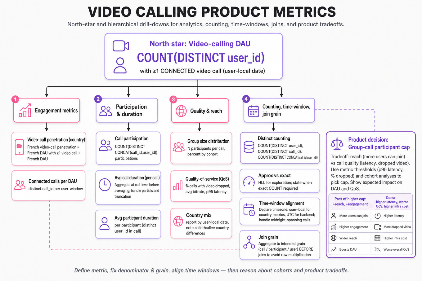
Interviewers are probing whether you can turn video-call event logs and user dimensions into reliable product metrics, then reason about trends, cohorts, and tradeoffs without overclaiming causality. For Meta, calling products are high-scale social surfaces where small metric definitions can change conclusions: `DAU`, call participation, call duration, country mix, group size, and quality-of-service all interact. A strong Data Scientist must define the denominator, join logic, time window, and segmentation before computing anything. The deeper version is deciding how a metric should guide product decisions, such as choosing a group-call participant cap that balances reach against call quality.

Core knowledge

• Metric definition is the first step, not an afterthought. For video calling, distinguish call_initiated, call_connected, participant_joined, participant_left, and call_ended. “Used video calling” usually means at least one connected video-call participation, not merely seeing or tapping the call button.

• Denominator discipline matters for percentages. A metric like French video-call penetration should usually be $\frac{\text{French `DAU` with ≥1 video call}}{\text{French `DAU`}}$ not calls divided by users, not video-call users divided by all global users, and not participants divided by `DAU` if the same user can appear multiple times.

• Distinct counting is central in calling analytics. Use COUNT(DISTINCT user_id) for users, COUNT(DISTINCT call_id) for calls, and sometimes COUNT(DISTINCT CONCAT(call_id, user_id)) for participations. At Meta scale, approximate methods like HyperLogLog may be used for exploration, but interview answers should state when exactness is required.

• Time-window alignment prevents silent bias. “Yesterday” needs a declared timezone, often user-local date for country-level product analytics or `UTC` for backend-consistent reporting. Cross-country comparisons can change if a call spans midnight or if caller and callee are in different countries.

• Join grain is the most common source of wrong answers. User tables are often one row per user, while call logs are many rows per call or participant. Joining a call-level table to a participant-level table can multiply rows; aggregate at the intended grain before computing avg_duration, `DAU`, or call counts.

• Duration metrics require clear semantics. Call duration may mean end-to-end call_end_ts - call_start_ts, connected duration only, or per-user watch/listen time. For group calls, total participant-minutes is \sum_i (\text{leave_ts}_i - \text{join_ts}_i) while call duration is max end minus min start; these answer different product questions.

• Country segmentation has edge cases. Country can come from profile, SIM, IP geolocation, or user-local locale; each has different noise. For cross-country calls, decide whether to attribute by caller country, callee country, all participant countries, or country-pair tuples like FR→US.

• Trend analysis should separate volume, rate, and composition. If video-call minutes rise in India, ask whether `DAU` rose, video-call penetration rose, calls per caller rose, or average duration rose. A useful decomposition is:
  $\text{minutes} = \text{DAU} \times \text{penetration} \times \text{calls per caller} \times \text{minutes per call}$

• Distribution analysis is often better than averages. For group-call participant caps, inspect percentiles such as p50, p90, p95, and p99 of max concurrent participants per call. Averages hide rare but important large calls; caps are naturally percentile-driven decisions.

• Quality tradeoffs should be quantified with an explicit objective. If `MOS` decreases with participant count, define an expected utility such as $U(k)=\text{covered calls}(k)-\lambda \cdot \text{low-quality calls}(k)$ or compare incremental reach from increasing cap k against incremental quality degradation.

• Causal claims need experimental or quasi-experimental support. Observing that longer calls increased after a launch is not enough; seasonality, country mix, holidays, or network conditions may explain it. For product changes, propose an `A/B` test with guardrails like crash rate, call setup failure, `p95` join latency, and negative social feedback.

• Small segments require uncertainty estimates. A country-date metric with few `DAU` can be noisy. For a proportion, use an approximate standard error $SE=\sqrt{\frac{p(1-p)}{n}}$ and avoid overinterpreting day-over-day swings where confidence intervals overlap.

Worked example

For Choose group-call participant cap via distribution, a strong candidate would start by clarifying the decision: “Are we choosing a hard maximum participant count for all users, or evaluating a default cap with exceptions for certain countries, devices, or network conditions?” They would also ask what the objective is: maximize successful group-call participation, preserve perceived quality measured by `MOS`, reduce call failures, or protect server/client performance as reflected in user-facing metrics.

The answer should be organized around four pillars. First, define the unit of analysis: one group call, with features like max concurrent participants, country mix, device class, network type, duration, and quality outcomes. Second, inspect the participant-count distribution: p50, p90, p95, p99, share of calls above candidate caps, and share of users affected. Third, model the quality relationship, for example estimating average `MOS` or call-failure probability by participant count while controlling for country, device, network, and call duration. Fourth, compare policies: cap at 8, 16, 32, or adaptive thresholds based on predicted quality.

The key tradeoff is that a cap may affect a tiny fraction of calls but a highly engaged or strategically important user segment. For example, a cap of 16 may cover 98% of calls, but if the remaining 2% are long, recurring community calls, the lost participant-minutes could be meaningful. A good candidate would avoid saying “choose p95” mechanically; instead, they would weigh marginal coverage against marginal quality degradation and propose guardrail metrics.

They should also flag that the observed historical distribution may be censored by the existing cap. If today’s product already limits calls to 16 participants, the data cannot reveal true demand above 16 without an experiment, waitlist, failed-invite data, or a temporary cap increase. A strong close would be: “If I had more time, I’d validate the recommendation with an `A/B` test that randomizes eligible calls or users to different caps, monitors `MOS`, join success, participant-minutes, retention, and complaint rates, and checks heterogeneity by market and network quality.”

A second angle

For Calculate Video Call Usage Metrics by Country and Date, the same skill set becomes more operational and metric-definition heavy. Instead of choosing a policy, the task is to produce a trustworthy country-date panel: date, country, `DAU`, video-call users, video-call user percentage, total video-call duration, and duration per `DAU`. The main constraint is grain: user activity is user-day level, while call logs may be call-level or participant-level. The candidate should explicitly avoid double-counting a user who joins multiple calls on the same date. The stronger answer also mentions that duration per `DAU` and duration per video-call user tell different stories: one captures overall product penetration, while the other captures intensity among adopters.

Common pitfalls

Pitfall: Using the wrong denominator.

A tempting answer is “French video-call percentage equals French video-call events divided by French `DAU`.” That is wrong if one user can generate many events. The better answer counts distinct French active users with at least one qualifying video-call participation and divides by distinct French active users.

Pitfall: Treating event timestamps as self-explanatory.

Candidates often compute “yesterday” with a raw event_timestamp filter and never discuss timezone, call-spanning behavior, or user-local dates. A stronger response says which date convention they are using and why, then notes how they would handle calls crossing midnight.

Pitfall: Jumping to causal product conclusions from descriptive cuts.

If cross-country calls are down 10%, it is not enough to say users dislike the product. A better answer decomposes the drop by `DAU`, penetration, calls per caller, duration, country-pair mix, app version, and quality metrics, then proposes an experiment or causal design only after ruling out obvious compositional and logging explanations.

Connections

Interviewers may pivot from this topic into experimentation design, especially how to test a new calling feature or participant cap with network effects and guardrail metrics. They may also ask about causal inference, metric design, retention analysis, or ranking/recommendation quality if calling entry points are surfaced by a recommendation system.

Further reading

• Trustworthy Online Controlled Experiments — Kohavi, Tang, and Xu — practical reference for `A/B` testing, guardrails, variance, and decision-making.

• Experimentation Works — Stefan Thomke — useful framing for product experimentation culture and interpreting evidence.

• The Signal and the Noise — Nate Silver — accessible treatment of uncertainty, forecasting, and overinterpreting noisy trends.

Practice questions

What's being tested

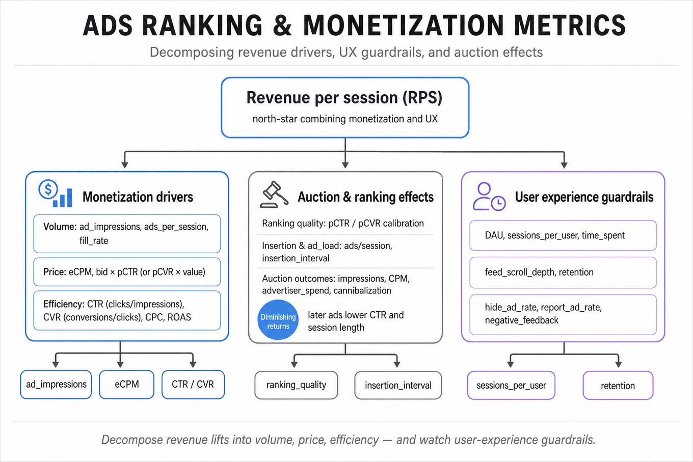
Meta ad ranking analytics tests whether a Data Scientist can reason about monetization, user experience, and causal measurement in the same system. Interviewers are probing for more than “revenue went up”: they want to see if you can define metrics, design a valid experiment, identify tradeoffs between ad load and engagement, and diagnose whether ranking changes improved the auction or merely shifted impressions. A strong answer connects ranking model quality, auction outcomes, advertiser value, and user retention without drifting into model-serving or data-pipeline implementation. Meta cares because small ranking or insertion changes can move billions of impressions while creating subtle harms: ad fatigue, advertiser budget cannibalization, short-term revenue spikes, or long-term feed engagement loss.

Core knowledge

• Ads ranking objective is usually some form of expected value:
  $\text{score} \approx \text{bid} \times P(\text{action}) \times \text{value adjustment} + \text{quality terms}$
  For click campaigns this resembles `eCPM` = bid_CPC × pCTR × 1000; for conversion campaigns it may use `pCVR`, predicted conversion value, and advertiser constraints.

• Primary monetization metrics should distinguish volume, price, and efficiency: `ad_impressions`, `clicks`, `conversions`, `CTR` = clicks / impressions, `CVR` = conversions / clicks or conversions/impressions, `CPC`, `CPM`, `eCPM`, `revenue_per_user`, `revenue_per_session`, and advertiser-side `ROAS`. A revenue lift alone is ambiguous without decomposing these drivers.

• User experience guardrails are essential because ads compete with organic feed content. Common guardrails include `DAU`, `sessions_per_user`, `time_spent`, `feed_scroll_depth`, `hide_ad_rate`, `report_ad_rate`, negative feedback, retention, and long-term engagement. A ranking change that increases `revenue_per_session` while reducing sessions can be value-destroying.

• Ad load is the number or density of ads shown per feed session, often expressed as `ads / feed_stories`, `ads / session`, or insertion interval. Revenue often has diminishing returns: the first extra ad may monetize well, but later ads can lower `CTR`, increase fatigue, reduce session length, or cannibalize higher-quality impressions.

• Auction and ranking effects must be separated from pure inventory effects. If revenue rises because users saw more ads, that is different from higher auction efficiency. Analyze normalized metrics such as `revenue_per_impression`, `eCPM`, `CTR`, `conversion_rate`, and user-level revenue, not just total revenue.

• Experiment unit choice is usually the user, not the impression, because impressions within a user are correlated and treatment changes future behavior. Randomizing at impression level can cause interference within a session and contaminate user experience metrics. Analyze at the user level when estimating standard errors.

• Power and minimum detectable effect matter because monetization metrics are often heavy-tailed. For a two-sample test, an approximate per-arm sample size is
  $n \approx \frac{2\sigma^2(z_{1-\alpha/2}+z_{1-\beta})^2}{\delta^2}$
  where $\delta$ is the detectable lift. Revenue may need winsorization, CUPED, or bootstrap confidence intervals.

• CUPED variance reduction uses pre-experiment covariates, often prior revenue or engagement, to improve precision:
  $Y_{adj}=Y-\theta(X-\bar X), \quad \theta=\frac{\text{Cov}(Y,X)}{\text{Var}(X)}$
  This is especially useful for ads because users have persistent monetization propensities.

• Attribution windows must be explicit for conversion metrics. A click-through conversion metric might count purchases within 1, 7, or 28 days after a click; view-through conversions are more vulnerable to correlation bias. State whether you measure same-session, same-day, or delayed outcomes.

• Heterogeneous treatment effects are central in ads. Segment by country, device, new versus mature users, session depth, advertiser vertical, campaign objective, and baseline ad engagement. A global average can hide harm to low-engagement users or over-monetization in sensitive markets.

• Interference and marketplace effects complicate experimentation. Changing ranking for treated users can alter advertiser budget pacing, auction prices, and availability for control users. For large marketplace changes, consider budget-aware analysis, geo-level tests, or limiting exposure to avoid cross-arm contamination.

• Tail and run analysis matters for insertion methods. Two systems with the same expected ad count can differ in the probability of consecutive ads, long gaps, or clusters. Metrics like probability of `2+` ads within `k` feed units, max run length, and distribution of inter-ad distance capture experience harms averages miss.

Worked example

For “Determine Key Metrics and Design A/B Test for Ad Ranking,” a strong first 30 seconds would clarify: what ranking change is being tested, whether the goal is advertiser value, Meta revenue, user experience, or a weighted objective, and whether the experiment affects ad selection, ad ordering, or ad load. I would state assumptions: randomize at the user level, keep ad load policy fixed unless explicitly part of the treatment, and evaluate both short-term monetization and engagement guardrails. The answer skeleton should have four pillars: define the objective and metrics, design the experiment, analyze heterogeneous effects, and make a launch recommendation.

For metrics, I would propose a primary business metric such as `revenue_per_user` or `revenue_per_session`, advertiser value metrics like `conversions_per_impression` and `ROAS`, and user guardrails such as `session_length`, `ad_hide_rate`, and retention. For design, I would use a randomized A/B test with pre-period balance checks, sample-size calculation, an experiment duration that covers weekday effects and delayed conversions, and user-level clustered standard errors. I would explicitly monitor `SRM`, pre-treatment covariate balance, and novelty effects, because ranking changes can cause early behavior shifts that do not persist.

One tradeoff I would flag is choosing `revenue_per_user` versus `revenue_per_impression` as the primary metric. `Revenue_per_user` captures total business impact, but it can rise from showing more or worse-timed ads; `revenue_per_impression` isolates auction efficiency but can miss user-level inventory changes. I would close by saying that if I had more time, I would estimate longer-term retention and advertiser budget effects, then run segment-level analyses to ensure the lift is not concentrated in a small high-monetization cohort while harming broader feed health.

A second angle

For “Determining the optimal ad load in News Feed,” the same concepts apply, but the treatment is not just ranking quality; it directly changes the quantity and spacing of ads. The key framing becomes marginal value: what is the incremental revenue from the next ad, and what is the incremental cost in engagement, retention, and advertiser performance? Instead of a single A/B test, I would consider multiple ad-load arms or a dose-response design, then estimate curves for `revenue_per_user`, `time_spent`, `hide_ad_rate`, and retention. The important constraint is nonlinearity: moving from 1 to 2 ads per session may be very different from moving from 6 to 7. I would also look for personalization opportunities because high-intent users may tolerate more ads while low-engagement users may churn.

Common pitfalls

Pitfall: Treating impressions as independent observations.

A tempting but wrong approach is to say, “We have billions of impressions, so the test will be powered immediately.” Impressions from the same user, session, advertiser, and auction are correlated, so standard errors can be severely underestimated. A better answer aggregates or clusters at the user level and discusses marketplace interference when advertiser budgets are affected.

Pitfall: Optimizing only for short-term revenue.

Saying “launch if `revenue` is statistically significantly positive” is incomplete. Ads ranking changes can increase near-term revenue by lowering relevance, increasing fatigue, or shifting spend from future auctions. A stronger recommendation balances `revenue_per_user`, advertiser outcomes, negative feedback, and retention, with a plan for longer-term monitoring.

Pitfall: Listing metrics without a decision framework.

Candidates often name ten metrics but never say which one decides launch, which are diagnostics, and which are guardrails. Interviewers want prioritization: one primary metric, a small set of guardrails with acceptable degradation thresholds, and diagnostic cuts that explain why the result happened.

Connections

Interviewers may pivot from ads ranking into incrementality measurement, uplift modeling, marketplace experimentation, or recommender-system evaluation. They may also ask SQL-style metric computation, but the Data Scientist expectation is usually to define attribution logic, denominators, and interpretation rather than design the underlying pipelines.

Further reading

• Trustworthy Online Controlled Experiments — Kohavi, Tang, Xu — Practical reference for experiment design, guardrails, variance reduction, and launch decision-making.

• The Unfavorable Economics of Measuring the Returns to Advertising — Lewis and Rao, 2015 — Explains why ad effects are hard to measure precisely, even with large samples.

• Position Auctions — Varian, 2007 — Useful background on auction mechanics and why ranking, bids, and predicted action rates interact.

Practice questions

What's being tested

Meta is testing whether you can turn an ambiguous product or integrity problem into a defensible measurement framework: north-star metric, input metrics, guardrails, cohorts, attribution rules, and diagnostic cuts. The interviewer is probing whether you understand the difference between “what we want to optimize,” “what we can reliably observe,” and “what could be gamed or biased.” For a Data Scientist, this matters because product decisions at Meta often depend on noisy behavioral data, heterogeneous user populations, network effects, and A/B tests where the wrong metric can push teams toward harmful local optima. Strong answers combine metric design, causal reasoning, statistical power, and practical diagnostics without drifting into implementation ownership.

Core knowledge

• North-star metrics should reflect durable product value, not just activity. For a community feature like `Circles`, a stronger primary metric might be meaningful creator-consumer interactions per active member, normalized by exposure, rather than raw posts or joins, which can be inflated by spam or low-quality activity.

• Metric trees separate outcome, input, and diagnostic metrics. Example: `B2B chat` success could use qualified conversation starts as an outcome, response rate and time-to-first-response as inputs, and blocked users, spam reports, or opt-outs as guardrails. This helps explain movement instead of only declaring “up” or “down.”

• Guardrail metrics protect user experience, integrity, and ecosystem health. Common guardrails include `hide_rate`, `report_rate`, `block_rate`, `unfollow_rate`, `session_length`, notification opt-outs, harmful-content prevalence, advertiser complaints, and support contacts. A launch should not rely on a positive primary metric if a guardrail shows practically meaningful harm.

• Normalization is essential when comparing groups with different opportunity sizes. Use rates like $\text{interaction rate} = \frac{\text{meaningful interactions}}{\text{eligible impressions or active users}}$ instead of raw counts. For creator/community products, consider per-capita, per-session, per-impression, and per-member denominators; each answers a different causal question.

• Cohorting and segmentation prevent averages from hiding product reality. Cut by new vs existing users, market, device class, language, creator size, business type, group size, spam-risk tier, and prior engagement. Meta interviewers often expect you to ask whether gains are broad-based or concentrated in a small, already-powerful segment.

• Attribution windows should match the product mechanism. A chat feature may need same-day response and 7-day retention windows; community features may need 14- or 28-day return behavior; harmful-content outcomes may require delayed labels. Too short a window misses downstream value; too long a window adds noise and confounding.

• Experiment design starts with unit of randomization. User-level randomization works for isolated experiences; community, page, advertiser, or thread-level randomization may be needed when there is interference between users. For networked products, define whether the estimand is direct effect, spillover effect, or total ecosystem effect.

• Power analysis matters for rare events like spam exposure or harmful-content reports. The approximate minimum detectable effect is proportional to $\text{MDE} \approx (z_{\alpha/2}+z_\beta)\sqrt{\frac{2\sigma^2}{n}}$. For very low base rates, consider aggregated exposure units, longer test duration, stratification, or higher-signal proxy labels.

• Proxy metrics are useful but dangerous. For harmful content, user reports are visible and timely but biased by user awareness, culture, language, and reporting propensity. Pair them with human review labels, classifier scores, prevalence estimates, and severity-weighted harm metrics rather than treating reports as ground truth.

• Severity weighting is often required for integrity measurement. A simple count of violations treats mild spam and severe abuse equally. A stronger metric is $\text{severity-weighted prevalence} = \frac{\sum_i \text{exposures}_i \times \text{severity}_i}{\text{total eligible exposures}}$, with transparent severity buckets and calibration checks.

• Diagnostic deep dives should follow a structured funnel: exposure → action → quality → retention → harm. If a metric drops, ask whether fewer users were eligible, fewer saw the feature, fewer acted after exposure, action quality changed, or downstream retention/harm shifted. This keeps diagnosis analytical rather than speculative.

• Data quality checks are in scope when framed as measurement validity. Before interpreting a movement, check logging coverage, denominator definitions, duplicate events, bot/spam filtering, experiment balance, sample-ratio mismatch, missing labels, and metric backfills. You do not need to design the ingestion system; you do need to know when measurement is untrustworthy.

Worked example

For “Define Success Metrics for Circle Feature Evaluation,” start by clarifying what `Circles` are meant to do: deepen meaningful interaction among a smaller group, increase retention, improve sharing comfort, or reduce broadcasting pressure. In the first 30 seconds, state assumptions: “I’ll treat this as a social/community product where success is not raw activity alone, but sustained high-quality engagement without safety or notification fatigue.” Organize the answer around four pillars: primary success metric, supporting funnel metrics, guardrails, and evaluation design.

A strong primary metric could be weekly active circle members with meaningful two-sided interactions, normalized by eligible users or circle members. Supporting metrics might include circle creation rate, invite acceptance, posting rate, comment/reaction depth, repeat participation, and 7-/28-day retention among creators and members. Guardrails should include hide/mute/leave rates, reports, blocks, notification opt-outs, and displacement from broader feed engagement. For evaluation, propose an A/B test if engineering allows randomization, with user- or circle-level assignment depending on spillovers; otherwise use a retrospective cohort design with matching or difference-in-differences.

Flag one explicit tradeoff: optimizing for circle posts may increase activity while fragmenting the broader social graph or increasing spammy invites, so the primary metric should require reciprocal or repeated engagement. Close by saying that with more time, you would validate whether the metric predicts long-term retention and run segment cuts for new users, highly connected users, small markets, and users with different baseline sharing behavior.

A second angle

For “Design harmful-content evaluation,” the same measurement discipline applies, but the objective shifts from growth to harm reduction under label uncertainty. Instead of a north-star like engagement, define severity-weighted harmful-content prevalence per impression or per user session, supported by detection rate, enforcement precision, appeal overturn rate, and time-to-action. The main constraint is that observed reports and takedowns are not the same as true harm; they are influenced by reporting behavior, model coverage, reviewer capacity, and adversarial adaptation. Experimentation also needs stronger guardrails: a ranking or enforcement change that reduces measured prevalence but suppresses benign content or disproportionately affects a language group may not be acceptable. The answer should emphasize calibration, bias checks, and severity tiers more than pure engagement lift.

Common pitfalls

Pitfall: Choosing a vanity metric as the primary success metric.

A tempting answer is “track number of messages,” “number of posts,” or “total reports removed.” These are easy to measure but do not prove user value or safety. A better answer ties the metric to the product goal and uses quality filters: qualified conversations, reciprocal interactions, severity-weighted exposure reduction, or retained active participants.

Pitfall: Skipping the denominator and cohort definition.

Saying “spam reports went up” is incomplete because it could mean more spam, better detection, higher user awareness, or more usage. Always specify the denominator, such as reports per eligible impression, per active user, or per conversation, and cut by cohorts with different exposure opportunities. This is especially important at Meta scale, where product changes often shift who is active, not just how active they are.

Pitfall: Treating metric design as a list instead of an argument.

A weak answer rattles off ten metrics without explaining why each one belongs. A strong answer says: “Here is the decision we need to make, here is the primary metric that maps to value, here are the guardrails that would block launch, and here are the diagnostics I would use if the result moves.” Interviewers reward structure because it mirrors how Data Science work influences real launch decisions.

Connections

Interviewers may pivot from metric design into A/B testing, causal inference, ranking evaluation, or integrity measurement. Be ready to discuss sample-ratio mismatch, heterogeneous treatment effects, CUPED variance reduction, proxy-label bias, and how offline model metrics like precision/recall connect to online product outcomes.

Further reading

• Trustworthy Online Controlled Experiments by Kohavi, Tang, and Xu — practical reference for experiment design, guardrails, power, and launch interpretation.

• Causal Inference for the Brave and True — accessible coverage of matching, difference-in-differences, instrumental variables, and observational evaluation tradeoffs.

• The Book of Why by Pearl and Mackenzie — useful conceptual grounding for causal graphs, confounding, and why correlation-based metrics can mislead.

Practice questions

Statistics & Math

What's being tested

Difference-in-Differences tests whether you can estimate causal impact when a clean randomized experiment is unavailable, using treated and comparison units observed before and after a launch. For a Meta Data Scientist, this matters because many product changes roll out by market, creator cohort, device type, country, or operational constraint rather than by user-level randomization. Interviewers are probing whether you can define the right estimand, build a valid panel, defend assumptions like parallel trends, and avoid common traps in staggered rollout analysis. They also want to see whether you can translate causal design into product metrics such as DAU, adoption rate, revenue per user, call creation, conversion, or retention.

Core knowledge

• Canonical DiD compares treated-unit changes to control-unit changes:
  $\hat{\tau}_{DID} = (\bar{Y}_{T,post}-\bar{Y}_{T,pre}) - (\bar{Y}_{C,post}-\bar{Y}_{C,pre})$
  It removes time-invariant group differences and common shocks, but only identifies causal effects under credible counterfactual trend assumptions.

• Parallel trends means treated and comparison units would have evolved similarly absent treatment. You cannot prove it, but you can diagnose it using pre-period event-study coefficients, placebo launches, matched comparison groups, and domain checks for seasonality, product eligibility, or launch targeting.

• Panel construction is often the hardest practical step. Build a unit-time dataset such as user_id × day, country × week, or group_id × month, with treatment date, outcome, covariates, exposure eligibility, and event time $k=t-G_i$. Aggregate before modeling when raw events are too granular.

• Two-way fixed effects models use unit and time controls:
  $Y_{it} = \alpha_i + \lambda_t + \beta D_{it} + \epsilon_{it}$
  Here $\alpha_i$ absorbs fixed unit differences and $\lambda_t$ absorbs global shocks. This is simple, but can be biased with staggered timing and heterogeneous effects.

• Staggered adoption means units enter treatment at different dates. A naive treated × post coefficient can compare newly treated units to already treated units, creating misleading or even negative-weight estimates when treatment effects vary over time or across cohorts.

• Modern staggered DiD usually estimates cohort-time effects $ATT(g,t)$, where $g$ is the first treatment period and $t$ is calendar time. Safer approaches compare each treated cohort to never-treated or not-yet-treated units, then aggregate with explicit weights.

• Event-study designs estimate dynamic effects around launch:
  $Y_{it} = \alpha_i + \lambda_t + \sum_{k \neq -1}\beta_k 1[t-G_i=k] + \epsilon_{it}$
  Pre-treatment $\beta_k$ values test trend plausibility; post-treatment $\beta_k$ values show ramp-up, novelty effects, decay, or delayed adoption.

• No anticipation requires units not to change behavior before treatment because they expect the launch. At Meta, this can fail if creators, advertisers, employees, or markets know a feature is coming, so exclude announcement windows or test for pre-launch movement.

• Stable Unit Treatment Value Assumption is fragile in social products. Network spillovers can occur when treated users affect untreated friends, groups, sellers, or viewers. If spillovers are likely, define units at a higher level, such as market or community, or interpret estimates as ecosystem-level effects.

• Inference should reflect correlation within units over time. Use cluster-robust standard errors at the treatment-assignment level, such as country, school, group, or user cohort. With few clusters, prefer wild cluster bootstrap or randomization inference over naive OLS standard errors.

• Metric design should separate exposure, adoption, engagement, and business outcomes. For example, track eligible_users, exposed_users, feature adoption, sessions, conversion, revenue, and guardrails like hide/report rate. DiD on a downstream metric is hard to interpret if eligibility or logging changes simultaneously.

• Robustness checks make the answer interview-grade: alternative control groups, different pre/post windows, placebo outcomes, leave-one-cohort-out analysis, covariate balance, seasonality controls, winsorization for heavy-tailed revenue, and segment cuts by market, platform, tenure, or baseline activity.

Worked example

For Derive and validate DID for staggered rollout, a strong first 30 seconds would clarify the unit of analysis, rollout rule, treatment date, outcome, and whether any units are never treated. You might say: “I’ll define treatment as first eligibility or first actual exposure, depending on the causal question, and build a unit-day panel with event time relative to rollout.” The answer should then organize around four pillars: estimand, identification assumptions, model specification, and validation. For the estimand, state whether you want the average treatment effect on treated units, $ATT$, or a dynamic effect by weeks since launch. For the model, avoid blindly defaulting to two-way fixed effects; explain that with staggered timing you would estimate cohort-time $ATT(g,t)$ using never-treated or not-yet-treated controls, then aggregate. For validation, show an event-study plot with pre-period coefficients, inspect whether treated cohorts were already trending differently, and run placebo treatment dates. A key tradeoff to flag is using not-yet-treated controls versus never-treated controls: not-yet-treated units may be more comparable but can be contaminated if they anticipate the launch. You would close by saying that, with more time, you would test robustness by cohort, platform, and baseline activity, and check whether spillovers violate the comparison group.

A second angle

For Evaluate shopping tab pre- and post-launch, the same causal structure applies, but the product framing is more metric-heavy. The interviewer likely expects you to define funnel outcomes such as tab impressions, product clicks, add-to-cart, purchases, seller revenue, buyer retention, and guardrails like session displacement or feed engagement loss. If the shopping tab launched by country or app version, DiD can compare changes in launched markets against similar not-yet-launched markets while controlling for global seasonality, holidays, and commerce trends. The extra challenge is attribution: revenue may move because of seller mix, promotions, supply changes, or logging updates, not just the tab. A strong answer would combine DiD with sensitivity checks, segment analysis, and a clear launch recommendation tied to both incremental value and metric reliability.

Common pitfalls

Pitfall: Treating pre/post movement as causal without a comparison group.

A tempting answer is “revenue increased 8% after launch, so the feature worked.” That ignores platform-wide shocks, seasonality, marketing campaigns, creator behavior, and macro trends. A stronger answer says the relevant quantity is the treated change minus the counterfactual change for comparable untreated or not-yet-treated units.

Pitfall: Using two-way fixed effects for staggered rollout without discussing heterogeneous effects.

Many candidates write $Y_{it}=\alpha_i+\lambda_t+\beta D_{it}$ and stop. That can be acceptable as a baseline, but it is incomplete when treatment effects vary by cohort or time since launch. Interviewers expect you to mention event studies, cohort-specific effects, and the risk of already-treated units acting as bad controls.

Pitfall: Over-focusing on formulas and under-explaining product validity.

A technically correct DiD can still be useless if treatment is defined incorrectly, the metric changed logging, or the control group was affected by spillovers. For Meta DS interviews, communicate the causal story: who was exposed, what behavior could change, what comparison is credible, and which guardrails prevent a false launch decision.

Connections

Interviewers may pivot from DiD into A/B testing, synthetic control, regression discontinuity, instrumental variables, or interrupted time series. They may also ask for SQL panel construction, metric instrumentation, power analysis under clustered assignment, or interpretation of an event-study chart with suspicious pre-trends.

Further reading

• Difference-in-Differences with Variation in Treatment Timing — Goodman-Bacon, 2021 — explains why naive two-way fixed effects can produce problematic weighted averages under staggered adoption.

• Difference-in-Differences with Multiple Time Periods — Callaway and Sant’Anna, 2021 — foundational paper for cohort-time $ATT(g,t)$ estimation.

• Estimating Dynamic Treatment Effects in Event Studies with Heterogeneous Treatment Effects — Sun and Abraham, 2021 — practical framework for event studies when rollout timing varies.

Practice questions

What's being tested

Meta Data Scientists are expected to reason from noisy user-level data to defensible product conclusions: estimate quantities like average comments per `DAU`, quantify uncertainty, compare model or product variants, and avoid false discoveries. Interviewers are probing whether you know when Central Limit Theorem approximations are valid, how to construct and interpret confidence intervals, how to handle skewed or count-based metrics, and how to design tests without inflating false-positive rates. They also care whether you can communicate assumptions clearly: independence, random sampling, treatment assignment, metric definition, and whether the uncertainty is statistical, measurement-related, or causal. Strong answers connect formulas to product decisions, such as whether a ranking change, comment composer tweak, or chatbot model is ready to ship.

Core knowledge

• Expectation is the long-run average of a random variable: $E[X] = \sum_x xP(X=x)$ for discrete outcomes. For user comments, the sample mean $\bar X = \frac{1}{n}\sum_i X_i$ estimates expected comments per user or per `DAU`, depending on the sampling unit.

• Sample variance uses $n-1$, not $n$, when estimating population variance from data: $s^2 = \frac{1}{n-1}\sum_i (X_i-\bar X)^2.$ Use the population standard deviation only when the full population distribution is known, which is rare in interview settings.

• Central Limit Theorem says $\bar X$ is approximately normal for large $n$ if observations are independent enough and variance is finite: $\bar X \approx N\left(\mu, \frac{\sigma^2}{n}\right).$ It can work well for user-level metrics with large `DAU`, but heavy tails and clustering slow convergence.

• A 95% confidence interval for a mean is commonly $\bar X \pm 1.96\frac{s}{\sqrt n}$ when $n$ is large. For small samples, use a t-interval: $\bar X \pm t_{0.975,n-1}\frac{s}{\sqrt n}$, especially if variance is estimated and normality is plausible.

• Count data like comments per user are often skewed, zero-inflated, and overdispersed relative to a Poisson model, where $E[X]=Var(X)$. A negative binomial or nonparametric approach is often more realistic if a few highly active users dominate variance.

• Bootstrap inference resamples users with replacement and recomputes the statistic, producing an empirical uncertainty distribution. For most interview-scale answers, 1,000–10,000 bootstrap replicates is enough; for very large samples, resample at the user level rather than event level to preserve the analysis unit.

• Independence is an assumption, not a given. User outcomes can be correlated through social graph effects, shared content, geography, or time shocks. If treatment is assigned by cluster, session, page, or conversation, standard errors must reflect that assignment unit.

• Power is the probability of detecting a true effect: $1-\beta$. For a two-sample mean comparison with equal group sizes, approximate required per-arm sample size is $n \approx \frac{2\sigma^2(z_{1-\alpha/2}+z_{1-\beta})^2}{\delta^2},$ where $\delta$ is the minimum detectable effect.

• Hypothesis testing separates effect size from uncertainty. A tiny lift in comments can be statistically significant with millions of users but product-irrelevant. Always report both the estimate and interval, for example “+0.3% comments per `DAU`, 95% CI [+0.1%, +0.5%].”

• Sequential testing requires a pre-planned correction if you repeatedly peek at results. Pocock boundaries spend alpha relatively evenly; O’Brien–Fleming boundaries are stricter early and closer to conventional thresholds later. Naively stopping when $p<0.05$ inflates false positives.

• Always-valid inference methods such as mixture SPRT, e-values, or confidence sequences allow continuous monitoring while controlling error rates under specified assumptions. In a DS interview, you do not need to derive them fully, but you should know why they avoid p-hacking better than ad hoc peeking.

• Joint probability questions often test whether you distinguish independence from correlation. If “honest” and “relevant” chatbot answers are independent, $P(H \cap R)=P(H)P(R)$; without independence, use $P(H \cap R)=P(H)P(R\mid H)$ and ask how labels were collected.

Worked example

For Analyze Central Limit Theorem in User Comment Distribution, a strong candidate first clarifies the sampling unit: “Are we sampling users from a day’s `DAU`, sessions, or comments? Is the target average comments per active user, total comments, or expected comments for a randomly chosen user?” They would declare assumptions: observations are user-level, sampled randomly from the relevant population, and each user contributes one count of comments for the day.

The answer should then be organized around four pillars. First, define the estimator: $\bar X$ estimates expected comments per active user, while $n\bar X$ estimates total comments for a population of size $n$ only if the sample represents that population. Second, discuss variability using $s/\sqrt n$, emphasizing that skewed counts can still have an approximately normal mean when $n$ is large. Third, build a confidence interval with either a normal or t critical value depending on sample size. Fourth, interpret the interval in product language: repeated samples would produce intervals covering the true mean about 95% of the time, not “there is a 95% probability this specific interval contains the truth.”

One tradeoff to flag is whether to rely on the CLT or use a bootstrap. If the distribution has many zeros and a few extreme commenters, the bootstrap may better reflect uncertainty for medians, percentiles, or trimmed means, while the CLT is still usually reasonable for the mean at large scale. A strong close would be: “If I had more time, I’d inspect the histogram, top-user contribution, day-of-week effects, and whether the target is user-level average or platform-level total.”

A second angle

For Apply sequential testing without p-hacking, the same uncertainty concepts apply, but the main risk shifts from estimating one interval to controlling error under repeated decisions. A candidate should immediately ask how often results will be checked, whether the stopping rule is pre-registered, and whether the metric is primary or one of many guardrails. Instead of a fixed-horizon $p<0.05$ test, they should propose an alpha-spending plan such as Pocock or O’Brien–Fleming, or an always-valid method if continuous monitoring is operationally necessary. The transferable idea is that uncertainty statements are only valid under their design assumptions; changing the stopping rule after seeing data changes the meaning of the p-value. The product framing is also different: early stopping may save users from a harmful launch, but it usually costs power or requires stricter evidence.

Common pitfalls

Pitfall: Treating the CLT as “the data are normal.”

The CLT is about the sampling distribution of the mean, not the raw distribution of comments. A count distribution can be extremely skewed while the mean is approximately normal; a better answer says, “The user-level counts are not normal, but $\bar X$ may be approximately normal if $n$ is large and dependence is limited.”

Pitfall: Giving a formula without defining the unit of analysis.

Saying $\bar X \pm 1.96s/\sqrt n$ is incomplete if $n$ might mean comments, users, sessions, or conversations. Meta interviewers expect you to anchor metrics to entities like user-day, `DAU`, treatment arm, or labeled chatbot response; otherwise your standard error may be artificially small.

Pitfall: Confusing statistical significance with launch readiness.

A $p$-value below 0.05 does not mean the effect is large, causal under all conditions, or safe for all segments. Stronger communication pairs the estimate with confidence intervals, practical significance, guardrail metrics, and whether the test design controlled for peeking or multiple comparisons.

Connections

Interviewers may pivot from here to A/B testing, causal inference, multiple hypothesis correction, metric design, or model evaluation for ranking and chatbot systems. Be ready to discuss variance reduction methods like CUPED, heterogeneous treatment effects across cohorts, and how offline evaluation metrics connect to online user outcomes.

Further reading

• Trustworthy Online Controlled Experiments — Kohavi, Tang, and Xu — Practical treatment of experimentation, metrics, power, and common online testing failure modes.

• All of Statistics — Larry Wasserman — Concise reference for estimation, confidence intervals, hypothesis testing, bootstrap, and asymptotic inference.

• Sequential Analysis — Abraham Wald — Classic foundation for sequential probability ratio testing and the logic behind valid early stopping.

Practice questions

Machine Learning

What's being tested

Interviewers are probing whether you can turn an ambiguous product or integrity problem into a defensible applied machine learning plan: define the prediction target, construct labels, choose features, evaluate offline and online, set decision thresholds, and monitor outcomes after launch. At Meta scale, a Data Scientist is expected to reason about model quality through business and user metrics, not just AUC, because targeting, ranking, fraud, and location inference all create asymmetric costs and feedback loops. Strong answers show statistical judgment: how you handle biased labels, calibration, uncertainty, subgroup performance, and tradeoffs between engagement, revenue, safety, privacy, and fairness. The interviewer is not looking for production pipeline architecture; they are looking for whether your modeling choices would lead to better decisions.

Core knowledge

• Problem formulation comes before model choice. State whether the task is classification, regression, ranking, uplift modeling, or multi-objective optimization. For rollout targeting, predicting “will use feature” is different from predicting “incremental lift if exposed,” which requires treatment-control data and estimates like $E[Y(1)-Y(0)\mid X]$.

• Label design is often the hardest part. A fraud label from chargebacks is delayed and biased toward detected fraud; a “home vs office vs public” label may rely on weak supervision from repeated nighttime presence, user-declared signals, or aggregate patterns. Always discuss label noise, time windows, leakage, and whether negatives are true negatives or merely unlabeled positives.

• Feature engineering should map to causal or predictive mechanisms. For ads or shopping ranking, useful DS-level features include user affinity, item quality, price competitiveness, historical conversion rate, seller reliability, freshness, social proof, and query/context match. For privacy-sensitive inference, prefer aggregated, coarse, consented, and non-identifying features over raw location traces.

• Train/validation/test splits must reflect deployment. Random splits can overstate performance when users, sellers, devices, or locations repeat across rows. Use time-based splits, user-level holdouts, seller-level holdouts, or geo-level validation when generalization across future behavior or unseen entities matters.

• Baseline models are essential. Start with interpretable baselines such as logistic regression, regularized linear models, or simple scorecards, then compare to XGBoost, random forests, or neural ranking models if nonlinear interactions matter. A complex model is only justified if it improves decision quality, calibration, subgroup robustness, or ranking metrics.

• Offline metrics should match the decision. For binary classification, report ROC-AUC, PR-AUC, precision, recall, false positive rate, false negative rate, and calibration. For ranking, use NDCG@K, MAP@K, MRR, expected revenue, conversion-weighted utility, and guardrails such as hide/report rates or buyer dissatisfaction.

• Cost-sensitive evaluation is critical when errors are asymmetric. Define expected cost:
  $\text{Expected Cost}(t)=C_{FP}\cdot FP(t)+C_{FN}\cdot FN(t)+C_{review}\cdot N_{review}(t)$
  Choose thresholds based on business harm, user harm, review capacity, or risk tier rather than maximizing accuracy.

• Calibration matters whenever scores drive thresholds, prioritization, or expected value. A calibrated model satisfies $P(Y=1\mid \hat p=s)\approx s$. Use reliability curves, ECE, Brier score, Platt scaling, isotonic regression, and segment-level calibration checks by country, device type, traffic source, seller size, or user tenure.

• Selection bias appears in ranking and rollout systems. Historical clicks and conversions are observed only for items users saw, so naïve training learns exposure policy artifacts. Discuss randomized exploration buckets, inverse propensity weighting, counterfactual evaluation, or interleaving tests when evaluating new ranking logic.

• Multi-objective ranking requires explicit utility design. For shopping, a score might combine predicted purchase value, user satisfaction, seller quality, integrity risk, and diversity:
  $S = w_1P(\text{purchase})\cdot \text{margin} + w_2P(\text{save}) - w_3P(\text{fraud}) - w_4P(\text{negative feedback})$
  A strong answer explains how weights are set, constrained, and tested.

• Fairness and subgroup analysis are model evaluation responsibilities. Check performance by protected or sensitive-adjacent groups where appropriate, plus operational segments like new users, small sellers, low-connectivity regions, and sparse-history users. Look for disparities in false positive rates, ranking exposure, calibration, and downstream outcomes.

• Online evaluation closes the loop. Offline wins do not guarantee product wins because models change user behavior. Use A/B tests with primary metrics, guardrails, ramp plans, novelty effects, and long-term holdouts where needed. Monitor drift in feature distributions, score distributions, calibration, precision at actioned thresholds, and product metrics after launch.

Worked example

For “Evaluate fraud classifier with cost-sensitive metrics,” a strong candidate would start by clarifying the action: are high-risk cases blocked automatically, sent to manual review, stepped up for verification, or merely downranked? They would ask what counts as fraud, how labels arrive, the delay in confirmation, the cost of a false positive to legitimate users, and the cost of a false negative to the platform. The answer can be organized into four pillars: label and data quality, offline model evaluation, threshold and decision policy, and online monitoring. For offline evaluation, they would not stop at ROC-AUC; they would emphasize PR-AUC if fraud is rare, precision/recall at operational thresholds, calibration curves, and segment-level false positive rates.

The candidate should define a cost function such as $C_{FP}$ for blocking a legitimate user, $C_{FN}$ for missed fraud, and $C_{review}$ for human review, then choose thresholds that minimize expected cost subject to capacity or safety constraints. A key tradeoff is whether to use a single global threshold or risk-tiered thresholds by transaction amount, account age, country, or seller history; tiering can improve utility but may create fairness and calibration concerns. They should also discuss delayed labels: recent “non-fraud” examples may simply not have matured, so evaluation should use a label window long enough to avoid optimistic estimates. They would close by saying that, with more time, they would run an online shadow test or limited ramp to compare modeled risk against actual downstream losses, user appeals, and support contacts.

A second angle

For “Optimize IG Shopping ranking with multiple objectives,” the same modeling-evaluation discipline applies, but the unit of decision is an ordered set of items rather than a binary action. Instead of choosing one fraud threshold, you are combining predicted purchase probability, long-term user satisfaction, seller quality, diversity, and integrity risk into a ranking objective. Offline metrics like NDCG@K or conversion lift are useful, but biased because historical exposure determines what outcomes were observed. A strong answer would introduce counterfactual evaluation, randomized exploration, and online A/B testing with guardrails such as user hides, seller concentration, refund rates, and low-quality purchase signals. The framing shifts from “minimize classification cost” to “maximize constrained expected utility under feedback loops.”

Common pitfalls

Pitfall: Optimizing for accuracy or ROC-AUC without connecting the metric to the decision.

This is especially weak for rare events like fraud or high-stakes targeting, where a model can achieve high accuracy by predicting the majority class. A better answer defines the action, the cost of each error, and the threshold or ranking policy that will be evaluated.

Pitfall: Treating observed labels as ground truth without discussing bias.

Clicks, conversions, fraud reports, and inferred place types are all partially observed and shaped by previous systems. Strong candidates explicitly call out delayed labels, missing positives, exposure bias, sample selection, and label noise, then propose practical mitigations like matured evaluation windows, audits, exploration data, or weak-supervision confidence scores.

Pitfall: Jumping to model architecture before framing the product and statistical problem.

Saying “I’d train XGBoost with many features” is not enough. Interviewers want to hear how you define success, prevent leakage, evaluate subgroups, calibrate probabilities, choose decision thresholds, and validate online impact.

Connections

This topic often pivots into experimentation, especially how to test a new targeting or ranking model with A/B metrics and guardrails. It also connects to causal inference for uplift modeling, metric design for multi-objective tradeoffs, and responsible AI for privacy, fairness, and subgroup reliability.

Further reading

• “Practical Lessons from Predicting Clicks on Ads at Facebook” — useful context on large-scale applied prediction, calibration, and feature/model tradeoffs in ranking-like systems.

• “Hidden Technical Debt in Machine Learning Systems” — explains why monitoring, feedback loops, and evaluation design matter beyond offline model performance.

• “A Survey of Methods for Explaining Black Box Models” — helpful for discussing interpretability and diagnostic analysis without over-indexing on model complexity.

Practice questions

Behavioral & Leadership

What's being tested

Meta is testing whether a Data Scientist can turn ambiguous, conflicting product evidence into a clear recommendation that cross-functional partners can act on. The interviewer is probing for more than “I ran an experiment”: they want to see how you define decision criteria, interpret heterogeneous metric movement, communicate uncertainty, and influence without authority. This matters because product launches often involve trade-offs across users, creators, advertisers, surfaces, or time horizons, and DS is expected to be the analytical lead who prevents teams from overreacting to one appealing metric. Strong answers show technical rigor, product judgment, and calm leadership under disagreement.

Core knowledge

• Decision framing comes before analysis. State the product goal, decision owner, launch options, primary metric, guardrails, and irreversible risks. A strong DS answer distinguishes “What is true?” from “What should we do given uncertainty, costs, and risk tolerance?”

• Metric hierarchy prevents cherry-picking. Use one primary success metric, such as sessions_per_user, 7d_retention, or revenue_per_impression, plus guardrails like hide_rate, report_rate, creator_posts, or long_term_value. If every metric is equally important, stakeholders will argue from whichever metric supports their preferred outcome.

• Experiment interpretation should include effect size, confidence, power, and practical significance. A result like $+0.3\%$ on DAU with $p<0.05$ may matter at Meta scale; $+5\%$ on a niche segment may be noise if underpowered. Use confidence intervals: $\hat{\tau} \pm 1.96 \cdot SE(\hat{\tau})$.

• Heterogeneous treatment effects are often the source of conflict. Segment by new versus tenured users, geography, device class, creator size, account type, or prior engagement. Avoid post-hoc overfitting: pre-specify key cuts where possible, and treat exploratory segments as hypotheses unless the effects are large and consistent.

• Cannibalization means a local lift may reduce value elsewhere. For example, a feature may increase time_spent on one surface while reducing feed_sessions, messages_sent, or engagement on another account owned by the same person. Evaluate user-level or ecosystem-level impact, not just per-surface lift.

• Interference and network effects complicate clean A/B tests. If one user’s treatment affects another user’s experience, standard SUTVA assumptions break. For social products, consider cluster randomization, ego-network analysis, geo-level tests, or directional triangulation from holdouts, while clearly stating residual uncertainty.

• Pre-commitment reduces launch-time politics. Before reading results, align on launch thresholds: e.g., launch if primary metric is $>+0.5\%$ and no guardrail is worse than $-0.2\%$ with statistically credible evidence. For ambiguous outcomes, define follow-up test, partial rollout, or no-launch criteria.

• Risk management is part of analytical leadership. Recommend full launch, staged rollout, holdout, rollback, or iteration based on downside severity. For high-risk surfaces, use ramp plans such as 1%, 5%, 25%, 50%, 100%, with monitoring of report_rate, crash_rate, unsubscribe_rate, or other relevant guardrails.

• Causal humility makes your answer more credible. Name plausible confounders, novelty effects, seasonality, logging gaps, and multiple comparisons. If the experiment ran during a holiday, outage, or major product launch, say how you would validate robustness before influencing a launch decision.

• Communication should match the audience. Executives need the decision, risk, and business/user impact in one slide. PMs need product trade-offs and next steps. Engineers need clear instrumentation concerns or ramp criteria. Legal, policy, or integrity partners need explicit harm and mitigation framing.

• Conflict resolution is not consensus-seeking at all costs. A strong DS surfaces the disagreement, identifies which assumption differs, proposes a falsifiable analysis, and sets a deadline for decision. If disagreement remains, escalate with a crisp recommendation and uncertainty bounds rather than letting debate stall.

• Impact quantification should connect analysis to outcomes. Translate metric movement into scale: “A $+0.4\%$ lift in weekly_active_users affects roughly X users weekly,” or “The gain is offset by a $-1.2\%$ drop in creator posting among small creators, which may harm supply over time.”

Worked example

For Communicate trade-offs and influence launch, start by framing the first 30 seconds around the decision: “I’d clarify the product goal, the launch deadline, whether the unit of decision is user, account, or surface, and which metric represents ecosystem value rather than local lift.” Then declare an assumption: the experiment shows a per-account lift on the treated surface but possible cross-account or cross-surface cannibalization. Organize the answer into four pillars: metric hierarchy, experiment readout, stakeholder alignment, and launch recommendation.

First, define the primary metric at the ecosystem level, such as user-level meaningful_interactions or 7d_retention, rather than only account-level engagement. Second, examine cannibalization by comparing total user activity across accounts or surfaces, not only treated-account activity. Third, quantify uncertainty: show confidence intervals, segment stability, and whether the negative signal is concentrated in high-value or vulnerable cohorts. Fourth, communicate the trade-off in decision language: “This is a local win but not yet an ecosystem win, so I recommend a staged rollout only if the user-level guardrail is neutral within our pre-agreed threshold.”

One explicit trade-off to flag is speed versus ecosystem risk. Launching fast may capture engagement gains, but if the lift comes from shifting attention away from another important surface, the apparent gain could be illusory. Close by saying: “If I had more time, I’d run a longer holdout or cluster-based test to measure persistence and spillovers, but given the current evidence I’d recommend either a constrained ramp with guardrails or another iteration before full launch.”

A second angle

For Decide under adverse signals and conflicts, the same skill applies, but the emphasis shifts from persuasion around trade-offs to decision-making under risk. Instead of a clean local lift plus cannibalization concern, imagine the experiment has mixed signals: primary metric up, report_rate or hide_rate also up, and PM/engineering pressure to launch before a planning deadline. A strong answer would pre-commit to thresholds, separate reversible from irreversible harm, and recommend a launch path proportional to risk. The framing should include “What would make me stop the rollout?” and “Which adverse signal is a true user harm versus an expected short-term adjustment?” The close should be decisive: do not hide behind “more analysis” if the situation requires a recommendation.

Common pitfalls

Pitfall: Treating the behavioral question as a personality story instead of an analytical leadership story.

A weak answer says, “I communicated clearly and got everyone aligned.” A stronger answer explains what evidence was disputed, how you decomposed the disagreement, which metric or causal assumption mattered, and how your recommendation changed the launch decision.

Pitfall: Over-indexing on statistical significance without product judgment.

A tempting answer is, “The p-value was significant, so I recommended launch.” That misses magnitude, guardrails, heterogeneity, novelty effects, and ecosystem impact. Better: “The primary metric was statistically positive, but the confidence interval on a key harm metric included a practically unacceptable downside, so I recommended a staged ramp.”

Pitfall: Being too passive in cross-functional conflict.

Do not say, “The PM wanted to launch, so I shared the dashboard and let leadership decide.” Meta expects DS to influence, not merely report. A stronger response is, “I wrote a one-page decision memo with the launch criteria, quantified risks, and my recommendation, then aligned PM and engineering on a rollback plan.”

Connections

Interviewers may pivot from this topic into experiment design, metric design, causal inference, or product sense. Be ready to discuss holdouts, guardrail metrics, heterogeneous effects, network interference, and how you would communicate a no-launch recommendation to senior stakeholders.

Further reading

• Trustworthy Online Controlled Experiments — Kohavi, Tang, and Xu — Practical reference for experiment interpretation, guardrails, ramping, and decision quality.

• The Data Science Handbook — Field Cady — Useful for framing the DS role as analytical problem solver and communicator, not just model builder.

Practice questions