Particle Filter Interview: Weight Collapse, Resampling, and Recovery
Quick Overview
Practice particle-filter interviews with checked weights, ESS and systematic ancestors, then explain why equal weights can conceal lost localization support. Primary references, original worked assets and explicit evidence boundaries support focused interview practice.
Particle filter interview questions often move from a familiar update equation to a harder diagnosis: the weights look healthy, but the robot is confidently wrong. Weight degeneracy, sample impoverishment and lost support are different failures. Resampling can equalize weights while making the represented state space less diverse. Recovery requires examining the proposal, motion and observation models, not repeatedly normalizing the same missing hypotheses.
The official course and implementation references below support the mechanics. The eight-particle example is original and was executed locally in Python; it is not a deployed localization result. Use PracHub's importance sampling exercise to practice explaining what the weights correct before tracing which ancestors survive.
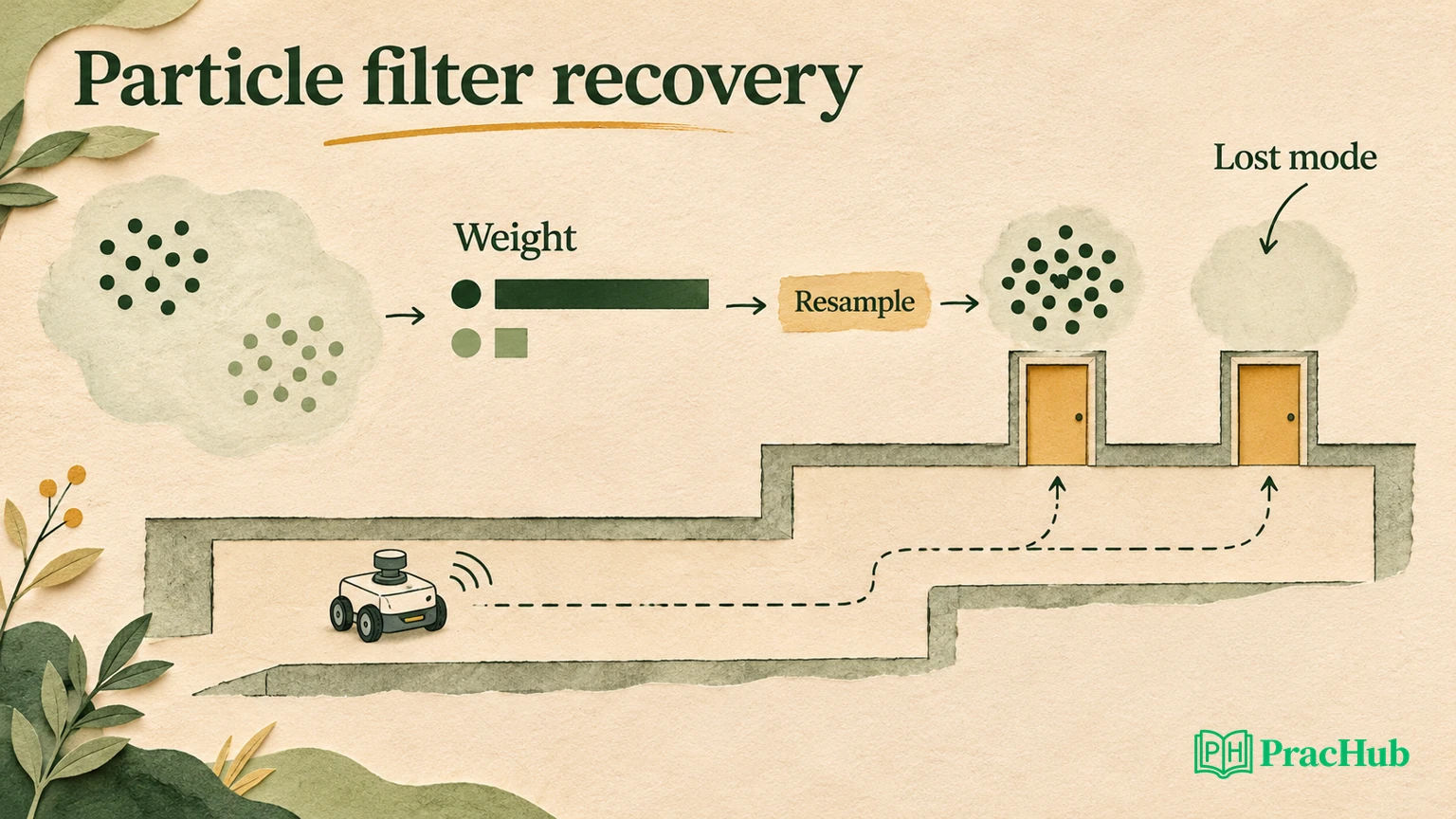
State what the particles and weights represent
A particle is a state hypothesis, such as a robot pose. Its weight contributes to a discrete approximation of the posterior. A cloud can represent several separated plausible locations, which is useful when a measurement has more than one explanation. The cloud's mean may lie between those locations and describe neither of them well.
The CTU autonomous robotics lesson describes prediction, observation weighting and resampling. For the original exercise, use a bootstrap proposal: sample motion from the transition model and multiply the previous weight by the observation likelihood before normalization. If the proposal differs, the general importance ratio must account for that difference.
bootstrap update:
    x[i] ~ p(x_t | x_previous[i], control)
    unnormalized[i] = previous_weight[i] * p(observation | x[i])
    weight[i] = unnormalized[i] / sum(unnormalized)
Do not omit the old weight unless a preceding step or another assumption makes it equal across particles. After ordinary resampling, equal starting weights make the likelihood-only shorthand appropriate for this update. Without that condition, replacing rather than multiplying weights changes the inference.
Ask which state dimensions the model includes, how controls enter, and whether the observation likelihood reflects sensor uncertainty and outliers. A correct resampler cannot compensate for a systematically incorrect likelihood that rewards the wrong location.
Calculate one deliberately uneven measurement update
Start with eight equally weighted particles at positions 0, 1, 2, 3, 6, 7, 8 and 9 meters. These are synthetic one-dimensional states, not a measured corridor. Supply likelihood scores 1, 1, 1, 1, 2, 4, 10 and 80. Only their relative values matter in this finite update.
Because the prior weights are equal, normalizing those scores gives:
| Particle index | State x | Likelihood score | Normalized weight |
|---|---|---|---|
| 0 | 0 | 1 | 0.01 |
| 1 | 1 | 1 | 0.01 |
| 2 | 2 | 1 | 0.01 |
| 3 | 3 | 1 | 0.01 |
| 4 | 6 | 2 | 0.02 |
| 5 | 7 | 4 | 0.04 |
| 6 | 8 | 10 | 0.10 |
| 7 | 9 | 80 | 0.80 |
The scores sum to 100. The common prior factor of 1/8 cancels during normalization. Show the normalization: calling a score a probability is unnecessary, and forgetting to normalize breaks later cumulative sampling.
A common effective sample size estimate is 1 / sum(weight[i] ** 2). Here the squared weights sum to 0.6524, giving ESS approximately 1.5328. The interpretation is that most normalized weight is concentrated in very few particles. It does not mean that exactly 1.5328 independent, accurate pose hypotheses exist.
If the interviewer suggests resampling below half the particle count, label that threshold as a chosen policy. It is not a universal correctness boundary. The cost of resampling, proposal quality and application requirements influence the policy.
Trace systematic resampling by hand
Official implementation reference: FilterPy's resampling documentation describes systematic resampling with one random offset and evenly spaced selection points. For eight samples, choose an offset in [0, 1/8). The original fixture fixes it at 0.03 so the result can be checked exactly.
The cumulative weights are 0.01, 0.02, 0.03, 0.04, 0.06, 0.10, 0.20 and 1.00. The selection points are 0.03, 0.155, 0.28, 0.405, 0.53, 0.655, 0.78 and 0.905. Choose the first cumulative value strictly greater than each point, using half-open intervals consistently.
import numpy as np

weights = np.array([.01, .01, .01, .01, .02, .04, .10, .80])
points = .03 + np.arange(8) / 8
ancestors = np.searchsorted(np.cumsum(weights), points, side='right')
# [3, 6, 7, 7, 7, 7, 7, 7]
The point exactly at 0.03 illustrates why boundary conventions matter in a deterministic demonstration. With the stated strict-greater convention it selects index 3. Random continuous offsets almost surely avoid exact boundaries, but a finite implementation still needs consistent behavior.
The new states are 3, 8, 9, 9, 9, 9, 9 and 9. Give each new particle weight 1/8. There are still eight particles, but only three distinct selected ancestors and three distinct state positions. Report copies and distinct hypotheses separately.
The local run checks these ancestor indices against the worked expectation. It is a finite reproducibility check, not a proof that systematic resampling is optimal for every distribution or that these eight particles represent the true posterior accurately.
Explain why ESS returns to eight without recovery
After equalizing weights, the ESS expression returns eight. Yet the particle at x = 1 has disappeared, and most particles occupy x = 9. Nothing about the equal weights proves that x = 9 is correct.
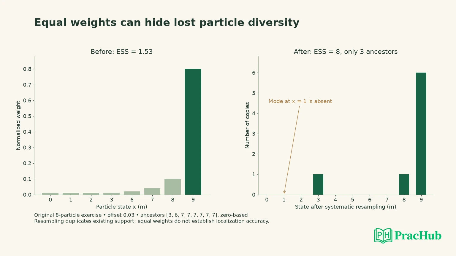
Separate the three failure types: Weight degeneracy concerns uneven weights. Sample impoverishment concerns repeated states or genealogies. Lost support means an important region has no useful representatives. One event can improve the first quantity while worsening the others.
Do not use unique-state count as the only replacement metric either. Continuous process noise can make every floating-point state distinct while all particles remain in the same incorrect region. Track spatial coverage, ancestor diversity, mode representation and observation consistency according to the problem.
A robot “kidnapped” to a distant location makes the support issue obvious. If all current particles and the motion proposal remain near the old location, weighting cannot create a particle at the new location. A sharp measurement may simply select the least-wrong old hypothesis and make the estimator look more confident.
Distinguish numerical repair from a missing hypothesis
Very small likelihood products can underflow. In the local example, exponentiating log weights −1000 and −1001 directly produces zeros in ordinary floating-point arithmetic. Subtracting the maximum before exponentiating yields normalized weights approximately 0.7311 and 0.2689.
m = max(log_weight)
scaled[i] = exp(log_weight[i] - m)
normalized[i] = scaled[i] / sum(scaled)
This repairs a finite numerical representation problem. It does not invent missing states, correct a bad sensor model or explain why a robot's observations disagree with every particle. If all log weights are negative infinity, subtracting the maximum also needs explicit handling; the simple finite example does not cover that case.
When all likelihoods collapse, inspect units, coordinate frames, timestamps, sensor saturation and outlier handling before blindly assigning uniform weights. Uniform weights over the same wrong particles can conceal the failure. Decide what state of uncertainty the application should report while evidence is insufficient.
Check accumulation across observations too. Multiplying many sharp likelihood terms may create overconfidence if the terms are correlated but treated as independent. Reducing numerical underflow does not make that independence assumption valid.
Design recovery as an explicit inference decision
Recovery can involve a broader motion proposal, observation-informed proposals, deliberate random reinjection or a reset under a recognized failure condition. These choices have different statistical meanings and computational costs. State whether the modification is an approximation, a heuristic or an importance-corrected proposal.
Official practical context: Nav2's AMCL configuration exposes particle and recovery-related parameters. Their existence does not imply that any one setting is suitable for every robot or map. Verify the installed version, configured behavior and failure case rather than copying a tuning value into an interview answer.
For the eight-particle case, explicitly injecting a new particle near x = 1 can restore representation of that region. It does not prove that x = 1 is true or that the resulting weighted cloud is an unbiased posterior approximation. The next observation must still discriminate among hypotheses, and the proposal treatment must be documented.
Roughening can separate duplicate particles locally, but it may not recover a remote missing mode. More particles can reduce sampling risk, but a larger population drawn from the wrong support remains wrong. These distinctions let you explain why a proposed recovery mechanism addresses a particular failure instead of treating every tuning knob as interchangeable.
Also define a runtime budget. Increasing particle count can delay updates, making the state estimate stale relative to the controller. A statistically richer cloud with unacceptable latency may harm the application. Report accuracy, uncertainty and timing together when evaluating a real implementation.
Show the evidence needed for a localization diagnosis
For an interview trace, log the pre-update cloud, observation timestamp, likelihood range, normalized weights, ESS before resampling, selected ancestor indices and resulting spatial coverage. Compare predicted observations with the actual measurement. This helps distinguish a sensor-model mismatch from a resampling implementation error.
Test a multimodal ambiguous observation, a discriminating observation, a corrupted observation and a sudden relocation. For the resampler, use a fixed offset to check exact indices, then varied seeds to study behavior across runs. A deterministic fixture and a statistical evaluation answer different questions.
The existing Kalman filter exercise develops Gaussian prediction and correction. The particle example adds a different concern: preserving or recovering plausible separated modes. Do not claim that switching from a Kalman filter automatically solves model mismatch or bad sensor timing.
When summarizing a failure, name the first broken assumption. “ESS is low” is an observation. “The likelihood rewards a mismatched map frame” is a hypothesis requiring a frame check. “Resampling erased a low-weight but important region” is a claim you can investigate with ancestor and state records.
Do not summarize a multimodal cloud with one confidence number
Consider two equally plausible groups on opposite sides of a map. Their weighted mean can fall in an empty or impossible location between them. Reporting only that mean and a post-resampling ESS discards the structure that made a particle representation useful. Preserve the modes or a suitable uncertainty summary for the consumer that needs to act.
The controller's response also belongs in the diagnosis. If localization has several separated hypotheses, the system may need to slow, stop, gather a discriminating observation or request relocalization. Which action is appropriate depends on the robot and its safety design. The filter's internal weight normalization alone cannot choose that policy.
During interview practice, ask what observation would separate the surviving hypotheses. A repeated ambiguous landmark may reinforce the same ambiguity, while a distinctive feature could resolve it. If no such observation is available, acknowledge the uncertainty rather than tuning the likelihood until one mode looks decisive. This connects the numerical trace to the actual purpose of state estimation without claiming a deployed recovery procedure.
Rehearse five related questions
These verified PracHub questions cover importance sampling, Bayesian updating, probabilistic modeling, possible positions and motion simulation. Some use different state spaces and are not dedicated particle-filter tasks. Apply the relevant reasoning without treating them as reported robotics employer prompts.
| PracHub question | Topic-specific rehearsal |
|---|---|
| Explain and derive importance sampling estimators | Explain the proposal correction and when old weights remain necessary. |
| How to Update Bayesian Model for Concept Drift? | Separate changed observations from an unsupported reset of the posterior. |
| Designing a Bayesian Classifier for Case Analysis | Discuss Bayesian evidence while acknowledging this classifier is not a particle filter. |
| Find possible robot positions | Distinguish possible positions from weighted state hypotheses and lost support. |
| Multi-Agent Collision Simulator (Unicycle Kinematics) | Keep motion-model assumptions separate from the observation likelihood. |
Return to the importance sampling question. Explain why old weights matter, compute the eight-particle update, and show why post-resampling ESS cannot establish recovery. Then propose one observation or proposal change that could restore useful support and state its remaining limitation.
Comments (0)