Power BI DAX Interview Questions: Filter Context, CALCULATE, and Correct Totals
Quick Overview
Practice Power BI DAX interview questions using six selected sales rows and sixteen executed DAX checks. Predict CALCULATE filter replacement, KEEPFILTERS intersections, REMOVEFILTERS scope, explicit and implicit context transition, distinct-customer totals, and weighted unit prices. Includes a runnable shared query and exact results.
Power BI DAX interview questions become easier when you explain the context before writing the formula. Which rows can the current filters reach? Which filter will CALCULATE replace? Is the requested total a sum, a distinct count, or a ratio that must be recalculated?
This guide answers those questions through six selected sales rows and sixteen executed DAX checks. The exercise and interview prompts are original preparation material, not claims about a particular employer’s question bank. Microsoft documentation supplies the language rules; the reported results come from actual DAX execution. For adjacent aggregation practice, use PracHub SQL aggregation questions.

Start with a model you can explain
We executed the complete verification query in DAX.do on September 9, 2026, using its DAX Guide model. The public query retains the six-row selection and all sixteen checks. This is DAX execution against an existing semantic model, not a Python emulation or a newly created Power BI Desktop report. The web interface did not expose an engine build number.
The relevant relationship is active and single-direction: Product[ProductKey] on the one side filters Sales[ProductKey] on the many side. We inspected the model diagram. Other dimensions exist in the hosted model; they are left unfiltered unless a test explicitly introduces a filter.
Official behavior: Relationships propagate filters between model tables. Their cardinality, direction, and active state affect that propagation; a relationship is not simply a SQL join pasted into a formula. See Microsoft’s model relationship guidance.
Our selected rows all belong to customer 18819 and store 199. Product 673 is Grey; product 560 is White. Both belong to Computers. Revenue is quantity multiplied by net price, so the discounted White item uses 152 rather than its 190 list price.
The first five lines belong to order 200710193CS570; the last belongs to 200712153CS570. Line numbers identify records within each order.
| Line | Product and color | Quantity × net price | Revenue |
|---|---|---|---|
| 78 | 673, Grey | 1 × 79 | 79 |
| 79 | 673, Grey | 1 × 79 | 79 |
| 80 | 673, Grey | 1 × 79 | 79 |
| 81 | 673, Grey | 3 × 79 | 237 |
| 82 | 673, Grey | 1 × 79 | 79 |
| 3 | 560, White | 1 × 152 | 152 |
The full query uses TREATAS on the six order-number/line-number pairs to keep every calculation within this scope. It does not replace the physical Product–Sales relationship. Microsoft documents TREATAS as applying table-expression values as filters to specified columns.
Do not select those order numbers and line numbers as independent lists: that loses the intended pairing. If you remove the six-row scope or run the measures over the entire hosted model, these example totals will change.
What is the current filter context?
Start with four measures. The shared query defines them with query-scoped MEASURE statements; the following snippets show their measure expressions:
Lab Revenue =
SUMX(Sales, Sales[Quantity] * Sales[Net Price])

Lab Units = SUM(Sales[Quantity])

Lab Customers = DISTINCTCOUNT(Sales[CustomerKey])

Lab Unit Price = DIVIDE([Lab Revenue], [Lab Units])
With only the six-row scope, revenue is 705, units are 8, and the distinct customer count is 1. A Grey filter on the Product table reaches five selected sales rows, whose quantities sum to seven and revenue to 553. White reaches the remaining row and returns 152.
Explain that a filter on Product[Color] restricts products, and the active relationship propagates that restriction to Sales. The measure then evaluates over the sales rows permitted by the combined context.
Ask where the filter originates. A filter on Product[Color], one on Product[ProductKey], and one on Sales[StoreKey] are different restrictions. Removing one column’s filter does not mean every remaining restriction disappears.
When does CALCULATE replace a filter?
Official rule: CALCULATE evaluates an expression in a modified filter context. A filter argument normally replaces an existing filter on the same column; it does not automatically erase unrelated filters. See Microsoft’s CALCULATE reference.
Suppose the outer context is Grey and this measure asks for White:
White Revenue =
CALCULATE([Lab Revenue], Product[Color] = "White")
In our six-row scope, it returns 152, not BLANK. The White restriction replaces the Grey restriction on the same color column. The explicit nested form used in the executed test makes the outer and inner contexts visible:
CALCULATE(
    CALCULATE([Lab Revenue], Product[Color] = "White"),
    Product[Color] = "Grey"
)
A strong follow-up answer names the boundary: this demonstration concerns a color-column filter. If an additional product-key restriction excludes the White product, replacing Color alone will not necessarily make that product available. Read the whole context before predicting the result.
CALCULATE changes context according to its arguments, so identify those arguments before explaining its effect on a slicer. You must identify the particular filter being added, replaced, or removed.
How do KEEPFILTERS and REMOVEFILTERS change the answer?
KEEPFILTERS makes the relevant filter combine by intersection with the existing filter. Microsoft’s KEEPFILTERS documentation describes this distinction explicitly.
White Within Selection =
CALCULATE(
    [Lab Revenue],
    KEEPFILTERS(Product[Color] = "White")
)
In a Grey-only outer context, the intersection is empty, so our revenue measure returns BLANK. Do not silently report zero as the observed result. Whether the report should display a zero is a separate presentation or business-definition decision.
REMOVEFILTERS clears the specified filter. Removing Color from the Grey context restores both selected products and returns 705:
Revenue Across Colors =
CALCULATE([Lab Revenue], REMOVEFILTERS(Product[Color]))
Compare the six primary executed cases:
| Context and calculation | Result | Reason |
|---|---|---|
| Six-row scope only | 705 | All selected revenue |
| Grey color | 553 | Five selected Grey rows |
| White color | 152 | One selected White row |
| Grey outside; White inside CALCULATE | 152 | Same-column replacement |
| Grey outside; KEEPFILTERS White inside | BLANK | Empty color intersection |
| Grey outside; REMOVEFILTERS Color inside | 705 | Color restriction cleared |
A seventh check adds Sales[StoreKey] = 306 before removing Color. All six rows belong to store 199, so the result remains BLANK. The store restriction survives. This is a concrete way to explain the scope of REMOVEFILTERS without saying it resets the entire report.
How does row context become filter context?
An iterator provides a current row, but that alone does not make every aggregation respect that row as a filter. This distinction is easier to see with a deliberately wrong expression:
SUMX(
    VALUES(Sales[ProductKey]),
    SUMX(Sales, Sales[Quantity] * Sales[Net Price])
)
Within our scope, VALUES(Sales[ProductKey]) contains two keys. The inner aggregation has no context transition tying it to the outer current key. It therefore evaluates the six-row revenue, 705, twice and returns 1,410.
Using the fact-side key list is intentional: it selects product keys present in the filtered Sales rows. With the model’s single-direction relationship, a Sales filter should not be assumed to restrict every row in the Product dimension. Microsoft’s VALUES reference explains that the returned values depend on the column’s filter context.
Add an explicit context transition:
SUMX(
    VALUES(Sales[ProductKey]),
    CALCULATE(
        SUMX(Sales, Sales[Quantity] * Sales[Net Price])
    )
)
The result becomes 705: 553 for one key plus 152 for the other. Calling the measure also returns 705:
SUMX(VALUES(Sales[ProductKey]), [Lab Revenue])
Microsoft documents that evaluating a model measure in row context performs context transition automatically. That is why replacing an inline aggregation with a measure can change the result. Do not explain the two forms as interchangeable solely because their arithmetic looks similar.
For interview practice, say which iterator creates row context, where context transition occurs, and which column value becomes a filter. Those three statements are more useful than memorizing “always add CALCULATE inside SUMX.”
Why is the distinct-customer total not two?
Each product’s selected sales involve the same customer, 18819. A product-level display therefore shows one customer for Grey and one for White. Across both products there is still only one distinct customer.
This expression returns two:
SUMX(VALUES(Sales[ProductKey]), [Lab Customers])
The expression is not a repair for an incorrect distinct-customer total. It calculates the sum of per-product customer counts, which counts this customer once for each product. That may be useful if the requested metric is customer–product participation, but it answers a different question.
Microsoft’s DISTINCTCOUNT documentation explains why distinct-count totals are non-additive. Before changing a measure, confirm whether the stakeholder wants unique customers across the selection or summed memberships across groups.
A concise answer could be: “The total of one is correct for unique customers. The visible rows overlap in customer identity. Summing them changes the metric to two product memberships.” This ties the DAX behavior to the business definition.
Which average should the total display?
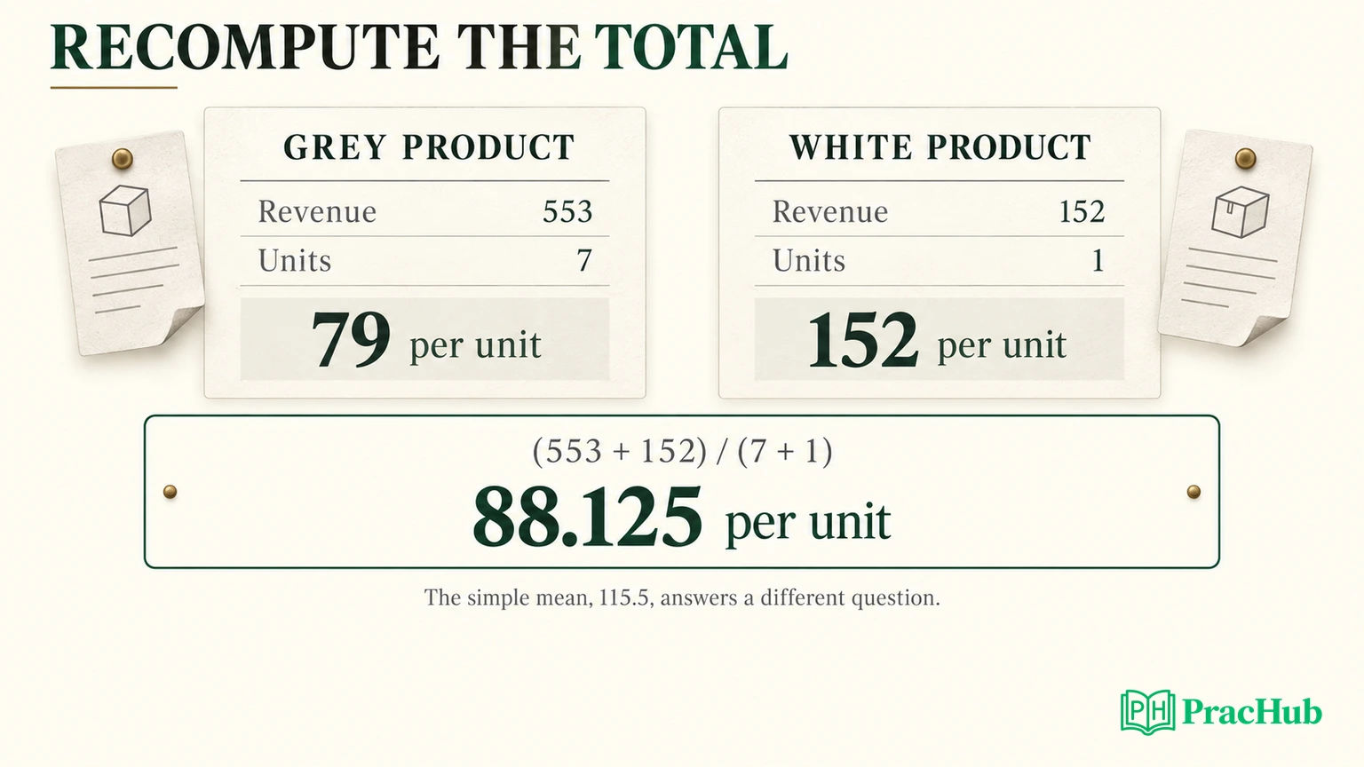
The two product-level realized unit prices are 79 and 152. Their simple mean is 115.5. But the selected sales contain seven units of the first product and one of the second.
For revenue per unit, calculate the ratio from its components:
DIVIDE([Lab Revenue], [Lab Units])
That is (553 + 152) / (7 + 1), or 88.125. A display formatted to two decimal places shows 88.13. The different display precision does not change the underlying business definition.
The executed alternative is:
AVERAGEX(VALUES(Sales[ProductKey]), [Lab Unit Price])
It returns 115.5, giving each selected product equal weight. Microsoft’s AVERAGEX reference describes an arithmetic mean over evaluated row expressions; the iterator’s grain determines what receives equal weight.
Neither number is inherently a DAX bug. For “realized revenue per unit,” 88.125 is the appropriate total. For “mean of the selected products’ realized unit prices,” 115.5 is appropriate. Ask the interviewer to confirm the intended denominator if the wording is ambiguous.
The same reasoning applies to rates and percentages. Retain the numerator and denominator measures so you can recompute the total in its own context. Microsoft’s DIVIDE reference also specifies the behavior for a zero denominator; define that case rather than relying on an accidental display.
Explain an unfamiliar measure before rewriting it
Use a short diagnostic sequence: identify the base grain and relationships, list active filters, locate context changes, state the metric definition, and predict a small counterexample. Then execute the measure and compare the actual output with that prediction.
The shared query provides sixteen results, including the six main filter states, a surviving store filter, three context-transition variants, distinct-count alternatives, average alternatives, and row/unit controls. All were run in DAX.do. The fixture does not validate your own model’s relationships, RLS, DirectQuery behavior, or Power BI visual configuration; those need separate checks in the target environment.
For adjacent practice, these verified PracHub questions develop aggregation, metric definition, and data-quality reasoning. They are not DAX runner exercises or claims about employer-specific DAX questions.
| PracHub question | What to practice |
|---|---|
| Write monthly customer and sales SQL queries | Keep customer identity, period, numerator, and denominator explicit. |
| Decide if subgroup increases imply overall increase | Explain how weights change an aggregate result. |
| Write SQL Data Transformation Queries | Separate row-level inputs from the requested aggregation grain. |
| Explain ETL schema changes and ensure integrity | Check whether upstream keys or data changes invalidate a model assumption. |
| Answer core behavioral questions for data roles | Describe a real metric-definition disagreement and how you resolved it. |
Continue with SQL aggregation practice on PracHub. For each result, explain which rows contributed and why the total answers the intended question.
Comments (0)