PromQL Interview Questions: Counter Resets, Vector Matching, and Histogram Queries
Quick Overview
Work through executable PromQL fixtures that expose aggregation-before-rate errors, missing label matches, and classic histogram percentile assumptions.
A PromQL query can return a plausible number and still answer the wrong question. Summing counters before calculating their rates, matching vectors on the wrong labels, or dropping a histogram boundary label can change the meaning without producing an obvious syntax error.
This guide uses original interview exercises executed with Prometheus promtool 3.14.0. Each exercise identifies its inputs, evaluation time, query, and expected result. Official documentation supports the language rules; the examples and explanations are editorial practice, not reports of a particular employer’s questions.
Start with Search Recorded Metrics by Name, Tags, and Recency to practice reading metric identity and labels before manipulating values. Here, that discipline is what separates a correct service rate from a misleading aggregate.
Read the metric type, labels, and time window first
For every question, state whether the input is a counter, gauge, or histogram; which labels identify a series; and whether the answer should retain instance-level detail. A suffix such as _total is a useful naming convention, but the producer’s metric definition determines its meaning.
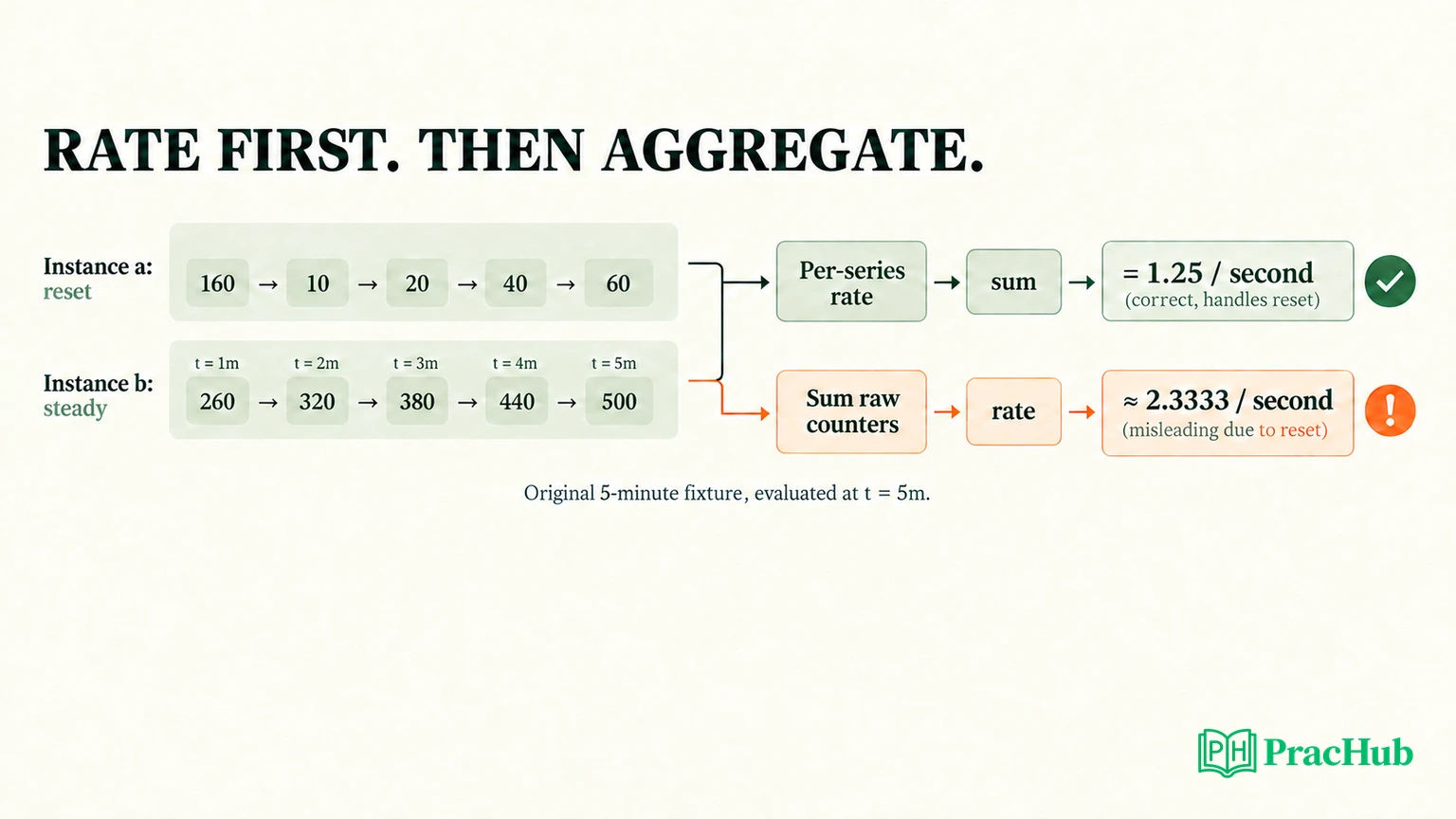
Our first fixture contains two counters named jobs_total. Both belong to service="api", with instances a and b. Samples occur every minute from t=0m through t=5m. The query is evaluated at t=5m with a five-minute range.
| Time | Instance a | Instance b | Raw sum |
|---|---|---|---|
| 0m | 100 | 200 | 300 |
| 1m | 160 | 260 | 420 |
| 2m | 10 | 320 | 330 |
| 3m | 20 | 380 | 400 |
| 4m | 40 | 440 | 480 |
| 5m | 60 | 500 | 560 |
Official semantics: a range selector excludes its left boundary and includes its right boundary. In this fixture, the [5m] range at t=5m includes the samples at minutes one through five, not minute zero. PromQL distinguishes instant and range vectors; a subquery is needed when you want a range of an expression’s results. Querying basics
That timing detail belongs in the answer. If you silently use all six samples, your arithmetic describes a different input window. Likewise, a five-minute graph range is not automatically the same thing as one instant evaluation over a five-minute selector.
Why calculate rate before aggregation?
Ask for the combined jobs-per-second rate across both instances. The intended query is:
sum by (service) (rate(jobs_total[5m]))
The verified output is {service="api"} 1.25. Instance a contributes 0.25 jobs per second and instance b contributes 1. The instance label disappears because the result groups only by service.
Official behavior: rate accounts for counter resets and extrapolates to the requested range boundaries. The functions documentation recommends applying rate before aggregation so resets remain detectable per input series. increase expresses the extrapolated increase over the range rather than a per-second value. Query functions
In the selected samples, a drops from 160 to 10. Its reset-adjusted increase across the observed four-minute span is 60; dividing by 240 seconds gives 0.25. The fixture’s boundary extrapolation preserves that rate. Its five-minute increase is therefore 75, not the raw endpoint difference of −100. We verified both results.
Now evaluate the tempting alternative:
rate((sum by (service) (jobs_total))[5m:1m])
This is valid syntax, but our verified output is approximately {service="api"} 2.3333. The subquery produces a raw aggregate every minute. When that aggregate drops from 420 to 330, rate interprets the drop as a reset of the aggregate counter, even though instance b never reset.
The problem is lost identity. Reset correction belongs to each counter’s history, and summing first destroys that history. Do not fix the discrepancy with a multiplier or by adjusting the expected answer to match the dashboard. Change the order of operations and explain what information the correct order preserves.
What does the reset fixture actually prove?
The fixture also evaluates resets(jobs_total{instance="a"}[5m]), which returns one. That supports the diagnosis within the selected window. It does not establish why the process reset: a restart, instrumentation change, or another producer behavior would need separate evidence.
A useful follow-up is to explain why this is not a general two-point difference formula. Real scrape spacing, missing observations, the available sample span, and boundary extrapolation affect the result. The clean one-minute fixture makes the counterexample reproducible; it does not remove those production considerations.
Here is a minimal executable test file for the correct service rate:
rule_files: []
tests:
- interval: 1m
  input_series:
  - series: 'jobs_total{service="api",instance="a"}'
    values: '100 160 10 20 40 60'
  - series: 'jobs_total{service="api",instance="b"}'
    values: '200 260 320 380 440 500'
  promql_expr_test:
  - expr: 'sum by(service)(rate(jobs_total[5m]))'
    eval_time: 5m
    exp_samples:
    - labels: '{service="api"}'
      value: 1.25
Save it as queries.yml and run promtool test rules queries.yml. Official tooling: promtool supports expression tests with input series, evaluation times, and expected samples. Its shorthand can express repeated increments, making compact fixtures possible. Unit testing for rules
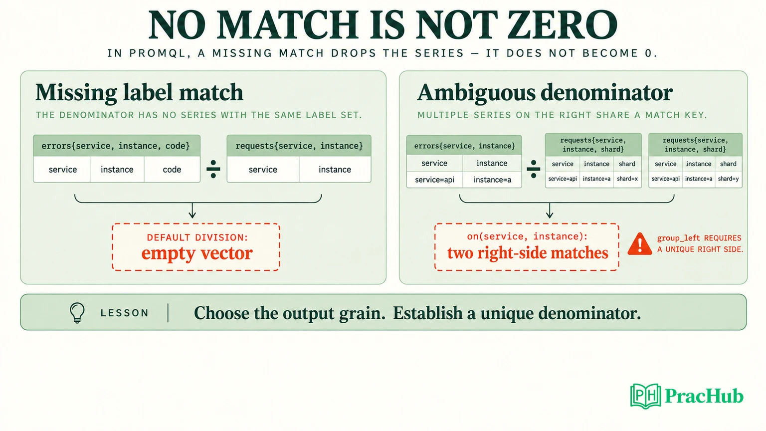
Why does a ratio return no series?
For the next fixture, use one-minute samples from t=0m to t=5m. errors_total has two series for service api and instance a: code 500 increases by six each minute; code 503 increases by three. requests_total increases by 600 each minute and has service and instance labels, but no code label.
Their rates are 0.1, 0.05, and 10 per second. This query returns an empty vector, not zero:
rate(errors_total[5m]) / rate(requests_total[5m])
The vectors do not have matching label sets. A missing result does not prove there are no errors, and converting it to zero would conceal the mismatch.
For an error ratio broken down by code, the verified correction is:
rate(errors_total[5m])
  / ignoring(code) group_left
rate(requests_total[5m])
The outputs retain service, instance, and code: code 500 is 0.01, and code 503 is 0.005. Those correspond to 1% and 0.5%. They use the same total-request denominator intentionally; they are contributions to the overall error ratio, not rates within separate status-code populations.
Official rules: ignoring excludes specified labels from matching, while on selects the matching labels. Group modifiers permit specified many-to-one or one-to-many arithmetic matches; the one-side match must remain unique. Operators
If the question instead asks for one service-wide error ratio, aggregate each side to that grain before division:
sum by(service)(rate(errors_total[5m]))
  / sum by(service)(rate(requests_total[5m]))
The result is approximately {service="api"} 0.015, or 1.5%. Our runtime represented it as 0.015000000000000003. That tiny floating-point difference is distinct from a wrong label match or incorrect denominator.
Why can group_left still produce a matching error?
Change the denominator fixture: requests are now partitioned into disjoint shards x and y, each increasing by 300 per minute. Both share service api and instance a. Matching only on service and instance leaves two right-hand series for the same key.
rate(errors_total[5m])
  / on(service,instance) group_left
rate(requests_total[5m])
We ran this intentionally broken case. promtool failed with a duplicate-right-series error explaining that many-to-many matching is not allowed. Adding a group modifier did not make an ambiguous denominator meaningful.
Because these fixture shards count disjoint requests, we can sum them into one denominator per service and instance:
rate(errors_total[5m])
  / on(service,instance) group_left
sum by(service,instance)(rate(requests_total[5m]))
The corrected code-500 output is 0.01. The explanation must include the disjoint-shard assumption. If x and y were replicas counting the same requests, summing them would double-count traffic; a syntactically valid query would still be wrong. Resolve metric ownership before choosing an aggregation.
Write a classic histogram query with its bucket labels intact
Our latency fixture has cumulative buckets for service api. Over each minute, the le="0.1" bucket gains 30 observations, le="0.5" gains 50, and le="+Inf" gains 60. All start at zero, and all use the same five-minute evaluation setup.
The bucket rates are 0.5, approximately 0.8333, and 1 observation per second. These are cumulative counts: the 0.5-second bucket already includes the observations in the 0.1-second bucket. Adding the three bucket rates would count some requests more than once.
For the 75th percentile, the executed query is:
histogram_quantile(0.75,
  sum by(service,le)(rate(latency_seconds_bucket[5m]))
)
It returns {service="api"} 0.4, measured in seconds. The target cumulative rate is 0.75. It falls between 0.5 at the 0.1-second boundary and 0.8333 at the 0.5-second boundary. Interpolating within that bucket gives approximately 0.4 seconds.
Official context: classic histogram quantiles are estimates based on bucket boundaries. Aggregating compatible bucket series before estimating a quantile is different from averaging already-calculated percentiles. Histograms and summaries
Retaining le is necessary for this classic-bucket expression. Also check that producers use compatible bucket boundaries and the same units. A number without those assumptions is not yet an interpretable latency percentile. The fixture gives a controlled estimate; it does not reveal the exact distribution of individual durations inside the bucket.
What changes for native histograms?
A native histogram carries histogram information within its samples rather than representing each bucket as a separate float series. Our additional executed fixture uses custom-bucket native histograms, with boundaries 0.1 and 0.5 seconds and an implicit final infinite bucket. It deliberately matches the classic fixture’s distribution. Native histogram specification
For that fixture, the query becomes:
histogram_quantile(0.75,
  sum by(service)(rate(latency_seconds[5m]))
)
There is no le grouping label. The verified result is again 0.4 seconds. The native input uses schema −53 with per-bucket increments 30, 20, and 10, not the cumulative classic increments 30, 50, and 60.
Do not generalize this numerical comparison to every native schema. Standard exponential buckets have different boundaries and interpolation behavior. In an interview, identify the representation first, then choose the query and explain the estimate. “Remove _bucket” is not a complete migration plan.
Explain your result as a small proof
Our verification used ten successful expression assertions across the main, corrected-matching, and native fixtures, plus one intentionally failing ambiguous-match case. The binary version was recorded and its official release checksum verified. These are local query-engine tests, not production scrape, dashboard, or alert-delivery tests. Prometheus downloads
Before presenting an answer, name the output labels, units, and missing-data behavior. Then identify one input change that would expose a wrong assumption: a reset on one instance, an extra denominator shard, or a different histogram layout. That turns memorized syntax into a defensible explanation.
| PracHub question | What to rehearse |
|---|---|
| Search Recorded Metrics by Name, Tags, and Recency | Treat labels and time as part of metric identity. |
| Design a Server Metrics Monitor | Define the signal before selecting an aggregation. |
| Debug Metrics Computed Before Filtering | Explain why operation order changes meaning. |
| Analyze end-to-end request latency | Interpret a latency estimate within its evidence limits. |
| Design a Low-Latency Metrics and Alerting Platform | Connect query correctness to monitoring design. |
These are related engineering practice prompts, not claimed PromQL questions from a specific employer. Try Debug Metrics Computed Before Filtering and explain the reset counterexample from input rows to output series.
Comments (0)