OpenAI Data Scientist Interview Prep Guide

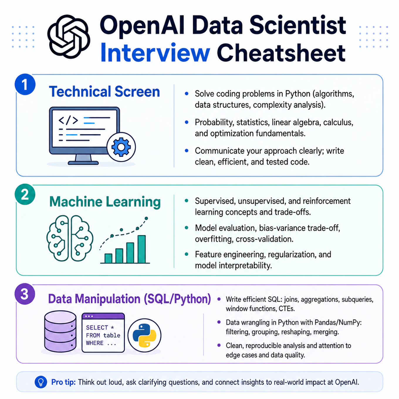
Focus most on the Technical Screen SQL/Python topics: cohort retention/churn SQL, event deduplication/data quality, and experiment-assignment reliability, since your Data Manipulation self-rating is 3/5 and you have viewed but not solved SQL/Python practice yet. Because all category self-ratings are 3/5 and there are no solved-question signals, nothing is treated as a proven strength; broader subscription experimentation and onsite PyTorch debugging stay lighter review. For OpenAI, the added emphasis is on LLM evaluation/safety metrics, model telemetry and inference-cost analytics, and human-feedback data quality rather than generic product analytics alone. With 1–2 weeks left, budget roughly 30 focused minutes for this cheatsheet pass, then spend most practice time writing SQL/Python aloud under timed conditions.

Technical Screen — 27 min

Machine Learning

Focus area — OpenAI data scientists need to connect usage, latency, token volume, reliability, and cost to product and model decisions.

What's being tested

The interviewer is probing your ability to treat model telemetry as measurable, testable signals: define robust metrics, detect and diagnose regressions, and quantify trade-offs between inference cost and model quality. They want to see statistical rigor (power, CIs, hypothesis framing), segmentation and causal reasoning (is cost change due to inputs, routing, or model change?), and pragmatic decisions for what to instrument and act upon at scale. OpenAI cares because inference costs are economically material and can interact with user experience in subtle, segment-specific ways.

Core knowledge

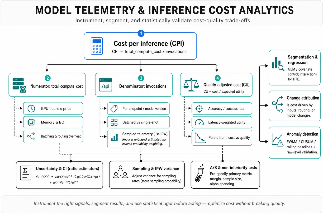
• Cost per inference basics: compute as $\text{CPI} = \frac{\text{total\_compute\_cost}}{\text{invocations}}$ and track aggregated and segmented CPI (by model version, endpoint, region, client).

• Latency distribution vs mean: track p50, p90, p99 (use quantile sketches like t-digest for streaming). Heavy tails can dominate cost and user experience despite benign means.

• Quality-cost tradeoff: evaluate cost-effectiveness via cost per correct prediction or cost-weighted utility: $\text{CU}=\frac{\text{cost}}{\text{expected utility}}$ and compare Pareto fronts across model variants.

• Ratio estimators & Delta method: for CPI or cost-per-success ratios, estimate variance with the delta method: $\text{Var}(\tfrac{X}{Y})\approx \frac{\text{Var}(X)}{\mu_Y^2} - 2\frac{\mu_X\text{Cov}(X,Y)}{\mu_Y^3} + \frac{\mu_X^2\text{Var}(Y)}{\mu_Y^4}$ for CI construction.

• Sampling and weighting: when telemetry is sampled, use inverse probability weighting (IPW) to recover unbiased estimates; ensure you know sampling rates and include them in variance estimates.

• A/B and non-inferiority tests: design tests with primary metric (e.g., accuracy, latency cost), choose margins for non-inferiority, compute sample size with variance estimates and desired power, and plan pre-specified stopping rules (alpha spending).

• Attribution via segmentation/regression: use stratified analyses and linear/GLM regressions with covariates (features, client, region, time-of-day) to control confounding when attributing cost changes. Consider interactions for heterogeneous treatment effects.

• Anomaly detection from a metric lens: detect change-points in aggregated metrics using rolling baselines, EWMA, or CUSUM with seasonality adjustments; validate with raw-level sampling to avoid false positives from aggregation artifacts.

• Micro vs macro telemetry: combine aggregated daily metrics (BigQuery, Postgres) with sampled request traces (Prometheus, logs) for debugging; treat traces as diagnostic samples, not population estimates unless sampling is known.

• Instrumentation for causal tests: prefer randomized assignment (A/B) to estimate causal cost impacts of model changes; where randomization is impossible, use difference-in-differences or instrumental variables with careful assumptions.

• Cost allocation & amortization: when GPU/CPU billing is per-hour, amortize cost across invocations using measured utilization (e.g., GPU-seconds) rather than wall-clock machine-hours to avoid misleading per-request CPI.

• Power & HTE planning: compute detectable effect sizes per segment; if small segments drive high costs, plan for targeted experiments or sequential buckets instead of one global test.

Worked example — "Investigate a sudden increase in inference cost while accuracy unchanged"

First 30s: clarify the signal (which cost metric rose? aggregated CPI, p99 latency, or GPU-hours?) and scope (single model version, region, or client subset), and ask about recent deploys or config changes. Skeleton approach: (1) validate telemetry and sampling rates, (2) segment by version/region/client/time and compute delta-CPI with CIs, (3) inspect request-level traces to find tail events, input-size shifts, or cache misses, (4) run regression to attribute cost to covariates (input length, prompt type, model routing), (5) simulate what-if: re-score historical requests against old/new model to confirm. A key tradeoff to highlight: full re-processing of historical traffic (gold standard) is accurate but expensive and slow; a targeted sample or cohort replay gives fast, lower-cost signals. Close by proposing immediate mitigations (roll back a suspect change, throttle expensive routes) and next steps: instrument finer-grained compute metrics and run an A/B to isolate cause.

A second angle — "Design an experiment to evaluate a lower-cost model variant"

Frame primary and secondary metrics up-front: a primary quality metric (e.g., task-specific accuracy or user engagement), and a primary cost metric (e.g., CPI or cost-per-success). Choose test type: non-inferiority if tolerating small quality drops for cost savings. Compute sample size using anticipated variance of the quality metric and the chosen non-inferiority margin; when cost is noisy, use stratified randomization by high-cost segments to ensure balance. Plan for heterogeneous treatment effects: predefine segment analyses, and adjust for multiple comparisons. Operational considerations: synchronous vs async routing, guardrails for high-cost outliers, and predefined interim analyses with alpha-spending to allow early stop for clear wins or losses.

Common pitfalls

Pitfall: trusting global means without checking tails.
If you report only average latency or CPI, you will miss rare, high-cost requests that can dominate billing or cause outages; always report p99/p999 and show distributional plots.

Pitfall: forgetting sampling design in metrics.
Telemetry traces are often sampled; treating trace-derived averages as population estimates yields biased CPI — always account for sampling probability with IPW and carry sampling uncertainty into CIs.

Pitfall: answering "why" with correlation not causation.
Pointing to input changes after a deploy is tempting, but without randomization or causal identification you must label findings as associative and propose causal checks (A/B, replay, IV) rather than assert direct attribution.

Connections

This topic naturally pivots to experimentation design (power, sequential testing), model evaluation (calibration, utility-weighted metrics), and anomaly detection for operational metrics. Interviewers may ask to expand into segmentation/Heterogeneous Treatment Effects or cost-aware optimization (constrained model training/pruning).

Further reading

• “Tail at Scale” (Jeff Dean et al.) — explains why tail latency matters and practical mitigation strategies.

• [Efron & Tibshirani, “An Introduction to the Bootstrap”] — concise guide to resampling CIs useful for complex telemetry estimators.

Practice questions

Focus area — Human evaluation data is OpenAI-specific enough to emphasize rater agreement, gold labels, bias, calibration, and annotation QA.

What's being tested

Interviewers probe your ability to measure, diagnose, and mitigate annotation noise so downstream model and experiment conclusions are valid. They want to see statistical rigor (inter-rater reliability, sampling variance), experimental design for labeling (stratified sampling, adjudication), and practical tradeoffs (cost vs. label quality, active relabeling). You are judged on framing clarifying questions, selecting appropriate metrics, running error-budget analyses, and recommending actionable next steps rooted in data.

Core knowledge

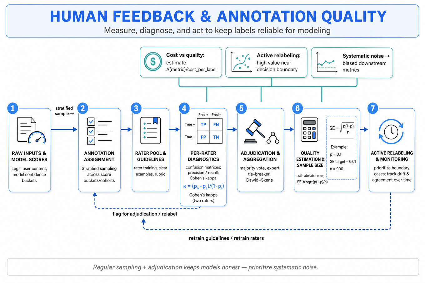
• Inter-rater reliability: common statistics are Cohen's kappa for two raters and Krippendorff's alpha for many/rate-variable tasks; Cohen's kappa = $(p_o - p_e)/(1-p_e)$ where $p_o$ is observed agreement, $p_e$ expected by chance.

• Confusion-matrix diagnostics: compute per-rater confusion matrices vs. a gold or majority label; derive precision/recall/F1 for each annotator to find systematic bias (e.g., conservative positive labeling).

• Sampling for quality estimation: use stratified sampling across model score buckets, user cohorts, or time to estimate label error rates with lower variance; compute margin using $SE \approx \sqrt{\hat{p}(1-\hat{p})/n}$ and choose $n$ to meet desired confidence.

• Adjudication workflows: common pipelines include majority-vote, expert adjudication (tie-breaker), and probabilistic label aggregation (Dawid–Skene) that estimate per-rater confusion matrices to produce latent true labels.

• Label noise models: model noise as class-conditional flip rates or rater-specific confusion matrices; recognizing non-random (systematic) noise matters more than i.i.d. noise for downstream bias.

• Impact on metrics: measurement error attenuates effects — estimated treatment effect $\hat{\tau}$ has extra variance and bias; when labels are noisy, power drops and Type I/II error rates shift.

• Cost-quality tradeoff: estimate value per reduced error (e.g., expected model metric improvement per additional high-quality label) and optimize budget across sampling, training, and adjudication.

• Online vs. offline label drift: track time-series of inter-rater agreement and label distributions; sudden shifts may indicate guideline drift or dataset distributional change requiring prompt retraining or guideline updates.

• Active relabeling: prioritize examples near decision boundary, high model uncertainty, or high disagreement among annotators for relabeling to maximize label-information per dollar.

• Calibration of evaluation: when creating evaluation sets, enforce label freeze, dedicated annotator pools, and document labeling spec to ensure reproducibility and guard against label leakage.

• Hypothesis testing under noisy labels: adjust variance estimates to account for annotation error; use bootstrap or simulation to measure the probability that observed metric deltas could arise from labeling noise.

• Metrics to monitor: track label_agreement_rate, per_label_precision/recall, annotator_completion_time, and annotation_spread (entropy across annotators) to diagnose quality and cost tradeoffs.

Worked example — "Design an annotation scheme and evaluate its quality for sentiment labels"

Frame: ask clarifying questions: what is the exact label granularity (binary vs. 5-point), who are annotators (experts vs. crowd), downstream use (training vs. evaluation), and budget/time constraints. Skeleton: (1) define a concise labeling spec with examples and edge cases, (2) pilot-label a stratified sample across domains and model-score buckets, (3) compute inter-rater agreement (Cohen's kappa or Krippendorff's alpha), per-class confusion matrices, and time/cost per label, (4) run an adjudication plan for disagreement cases and estimate post-adjudication label quality and remaining error. Tradeoff: explicitly flag the choice between finer granularity (more informative but lower agreement) and coarser labels (higher agreement but less signal for modeling). Close: propose concrete next steps — increase pilot size if CI wide, run active relabeling on model-uncertain examples, and if time permits, test how model metrics change when trained on adjudicated vs. raw labels.

A second angle — "Diagnose low agreement in human annotations"

Ask if low agreement is uniform across classes, annotators, or data slices. Evaluate per-example disagreement entropy and per-annotator confusion matrices to separate problematic examples (ambiguous content) from problematic annotators (systematic misunderstanding). Consider whether the labeling spec lacks clarity for specific edge cases, whether samples contain adversarial or off-domain content, or whether task cognitive load/time correlates with disagreement. Recommend targeted interventions: refine spec with clear examples, re-train annotators on failure cases, shift to coarse labels for ambiguous slices, or introduce expert adjudication only for contentious subsets.

Common pitfalls

Pitfall: Treating low agreement as purely "bad" and immediately firing annotators — often the root is an ambiguous spec or inherently subjective data; diagnose per-slice disagreement first.

Pitfall: Relying only on overall agreement metrics (e.g., percent agreement) — these mask class imbalance and chance agreement; always report chance-corrected statistics like kappa or alpha.

Pitfall: Ignoring sampling variance when comparing label quality across conditions — failing to compute confidence intervals can lead to overconfident decisions about who is "good" or whether a change improved quality.

Connections

Interviewers may pivot to active learning strategies for label efficiency, fairness and bias analysis when annotations differ across demographic groups, or A/B testing measurement when labels are used to compute product metrics. Be ready to link annotation quality improvements to model evaluation and experiment sensitivity.

Further reading

• Dawid, A. P., & Skene, A. M. (1979) — seminal probabilistic model for aggregating noisy categorical labels (Dawid–Skene).

• Krippendorff, K. (2011). Content Analysis: An Introduction to Its Methodology — authoritative discussion of reliability statistics and their interpretation.

Practice questions

Data Manipulation (SQL/Python)

This is in the canonical Technical Screen section, and you have viewed SQL/Python material but have no solved signal yet.

What's being tested

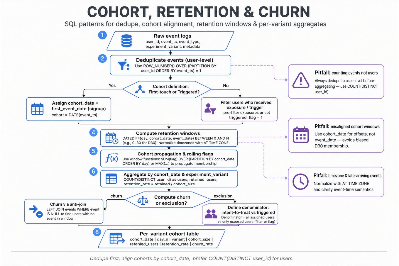
Demonstrates manipulation of SQL event-level logs to construct cohort analysis, compute retention and churn, and produce per-variant aggregates. Interviewer probes deduplication, time-windowing, correct cohort alignment, and clear assumptions about first-touch vs. triggered cohorts.

Patterns & templates

• ROW_NUMBER() for deduplication — use ROW_NUMBER() OVER (PARTITION BY user_id ORDER BY event_ts) to pick first/last event per user.

• Window functions for rolling/cohort flags — SUM(...) OVER (PARTITION BY cohort ORDER BY day) or MAX(...) to propagate cohort membership.

• Date arithmetic for retention windows — DATEDIFF(day, signup_date, event_date) BETWEEN 0 AND 30 for D30 retention; watch timezone.

• COUNT(DISTINCT ...) for unique-user metrics; prefer approximate (hyperloglog) only for very large cardinalities.

• Anti-join / LEFT JOIN ... WHERE null to compute churn/exclusion (users who didn’t convert or perform event).

• Intent-to-treat vs triggered — define the denominator: all assigned users vs. only those who received exposure; implement with pre-filtering or flags.

• Aggregate by variant/date — group by experiment_variant, cohort_date and compute rates with SUM(events)/COUNT(users); include NULL-handling.

Common pitfalls

Pitfall: Counting events instead of unique users — leads to inflated retention; always dedupe on user-level before aggregating.

Pitfall: Misaligned cohort windows (using event_date instead of signup_date) — yields wrong D30 membership and biased churn.

Pitfall: Ignoring late-arriving events or timezone differences — clarify event-time semantics and apply AT TIME ZONE or consistent normalization.

Practice these

The practice cards below cover the canonical variants — solve all of them and time yourself.

Practice questions