TikTok Data Scientist Interview Prep Guide

Technical Screen

Data Manipulation (SQL/Python)

• SQL Window Functions And Analytical Querying — covered in depth under Take-home Project below.

Analytics & Experimentation

• Cohort, Retention, Funnel And Product Metrics — covered in depth under Onsite below.

• A/B Testing And Experiment Design — covered in depth under Onsite below.

Statistics & Math

• Experiment Diagnostics, Power And Robust Inference — covered in depth under Onsite below.

• Propensity Score Matching, DiD And Causal Inference — covered in depth under Onsite below.

Machine Learning

• Recommendation, Ads Ranking And Marketplace Objectives — covered in depth under Onsite below.

• Classification Thresholds, Imbalanced Learning And Risk — covered in depth under Onsite below.

• Supervised ML Workflows, Interpretability And Deployment — covered in depth under Onsite below.

Behavioral & Leadership

• Behavioral Communication And Stakeholder Leadership — covered in depth under Onsite below.

Onsite

Data Manipulation (SQL/Python)

• SQL Window Functions And Analytical Querying — covered in depth under Take-home Project below.

Analytics & Experimentation

What's being tested

Interviewers are probing whether you can turn messy user-event data into defensible cohort, retention, funnel, and product metric conclusions. For TikTok, this matters because small changes in posting, viewing, shopping, or ad-load behavior can affect creator supply, viewer engagement, and monetization simultaneously. A strong Data Scientist should define the right denominator, align events in time, segment users meaningfully, and distinguish metric movement from causal impact. Expect to explain both the analysis logic and the business interpretation, not just write a query.

Core knowledge

• Cohort analysis groups users by a shared starting condition, usually first registration, first post, first purchase, or first exposure date. The most common cohort key is DATE(MIN(event_ts)) per user_id; always clarify whether the cohort is based on signup, first activity, or experiment assignment.

• Retention rate measures whether users return after an anchor event. For day-$N$ retention:

  $$D_N\ retention = \frac{\#\ users\ active\ on\ cohort\ date + N}{\#\ users\ in\ cohort}$$

  Clarify whether “active” means opening the app, watching, posting, liking, purchasing, or any qualifying event.

• Rolling retention and bounded retention answer different questions. Day-7 exact retention counts users active exactly on day 7, while 7-day rolling retention counts users active any time from day 1 through day 7. TikTok-style engagement analyses often need both because habit formation and occasional usage behave differently.

• Funnel analysis tracks ordered conversion through steps such as view_item → add_to_cart → purchase or video_view → profile_visit → follow. Define whether the funnel is user-level, session-level, or item-level; conversion rates change dramatically depending on that unit.

• Temporal ordering is essential in funnels. Use event timestamps and patterns like ROW_NUMBER() OVER (PARTITION BY user_id, product_id ORDER BY event_ts) to deduplicate repeated events, then require step $k+1$ to occur after step $k$. Counting unordered events creates inflated conversions.

• Metric decomposition separates topline movement into interpretable components. For ad revenue, a useful identity is:

  $$Revenue = DAU \times sessions/user \times impressions/session \times fill\ rate \times eCPM$$

  This lets you diagnose whether revenue changed because of traffic, ad load, auction pricing, or engagement.

• DAU growth vs monetization tradeoffs require both guardrail and objective metrics. A growth feature might increase DAU but reduce ARPDAU, session depth, or creator posting. A monetization change might increase ad_revenue but hurt watch_time, retention, or long-term user value.

• Segmentation is not optional. Retention and funnel behavior differ by new vs existing users, creator vs viewer, geography, device, traffic source, content vertical, and user maturity. A flat average can hide Simpson’s paradox, especially when traffic mix shifts across regions or acquisition channels.

• Causal inference matters whenever you interpret metric changes. If a cohort has higher retention after a launch, ask whether it was exposed to a treatment, acquired through a different channel, or affected by seasonality. Prefer randomized A/B tests; otherwise consider difference-in-differences, matching, or regression adjustment.

• Censoring and incomplete windows can silently bias retention. If today is 2026-05-23, users acquired on 2026-05-20 cannot yet have day-7 retention. Exclude immature cohorts from day-$N$ calculations or mark them incomplete instead of treating missing activity as non-retention.

• Statistical uncertainty should accompany metric reads. For a binary retention metric, a rough standard error is $\sqrt{p(1-p)/n}$; for funnel rates, compare proportions with confidence intervals or logistic regression. With very large samples, focus on practical significance, not only tiny p_values.

• Deduplication and event definition are analysis-layer responsibilities. If users can post multiple times or fire duplicate click events, decide whether to count distinct users, distinct sessions, or total events. For example, COUNT(DISTINCT user_id) answers active users; COUNT(*) answers total activity volume.

Worked example

For Analyze Trade-off Between DAU Growth and Ad Revenue, a strong candidate would start by clarifying the setup: “Are we evaluating an experiment, an observed trend, or a proposed product change? Are DAU and ad revenue measured globally or by market, and over what time horizon?” Then they would define the primary metrics: DAU, ad_revenue, ARPDAU, retention, watch_time, ad_impressions_per_user, and possibly creator-side metrics if the feature affects posting supply.

The answer should be organized around four pillars. First, decompose revenue into traffic, engagement, ad inventory, fill rate, and price, so the tradeoff is not treated as one black-box number. Second, segment by user maturity, geography, acquisition source, and engagement level to see whether growth comes from low-monetizing or high-retaining users. Third, evaluate causality with an A/B test if available, using DAU or retention as engagement metrics and revenue per eligible user as monetization metrics. Fourth, make a decision framework: launch if long-term engagement gain outweighs short-term revenue loss, but block if guardrails like day-7 retention, session length, or ad fatigue degrade materially.

One explicit tradeoff to flag is short-term versus long-term value. Increasing ad load may raise same-day revenue while reducing future retention; reducing ad load may lower ARPDAU today but increase future LTV. A strong close would be: “If I had more time, I’d estimate cumulative 7-, 14-, and 28-day revenue and retention by cohort, not just same-day DAU, because this decision depends on lifetime value rather than a single-day metric.”

A second angle

For Calculate User Registration Date and 7-Day Retention Rate, the same core concept becomes more operational and cohort-oriented. Instead of debating business tradeoffs, the candidate must define each user’s registration or first activity date, assign them to a cohort, and check whether they performed a qualifying action exactly seven days later or within a defined 7-day window. The main constraint is precision: registration_date, timezone, event type, and inclusion of incomplete cohorts must be handled consistently. The interviewer is likely testing whether you can translate a product definition into a reproducible metric while avoiding denominator leakage. The best answer still includes interpretation: day-7 retention is not just a query output; it tells whether new users are forming a habit.

Common pitfalls

Pitfall: Treating event counts as user counts.

A tempting wrong answer is to compute retention as COUNT(posts_on_day_7) / COUNT(posts_on_day_0). That measures posting volume, not retained users, and heavy posters will dominate the metric. A better answer uses COUNT(DISTINCT user_id) for retention and separately reports posts per retained user if activity intensity matters.

Pitfall: Ignoring time alignment and cohort maturity.

Candidates often include users who have not yet had enough time to reach day 7, which mechanically depresses recent cohort retention. State that you would filter to cohorts with cohort_date <= current_date - interval '7 days' and align timestamps to the product’s reporting timezone before aggregating.

Pitfall: Jumping to a launch recommendation without diagnosing the metric movement.

For a DAU versus ad revenue question, saying “choose revenue because it is business-critical” or “choose DAU because growth matters” is too shallow. A stronger response decomposes the metrics, checks user segments, estimates long-term impact, and frames the decision around objective metrics plus guardrails.

Connections

Interviewers may pivot from here into experiment design, especially choosing primary metrics and guardrails for an A/B test. They may also ask about causal inference, ranking/recommender evaluation, or metric anomaly diagnosis, such as explaining why DAU rose while retention fell.

Further reading

• Trustworthy Online Controlled Experiments — practical reference for experiment metrics, guardrails, and decision-making.

• Causal Inference: The Mixtape — useful grounding for interpreting non-randomized cohort and retention differences.

• Lean Analytics — accessible product-metric framing across growth, retention, and monetization.

Practice questions

What's being tested

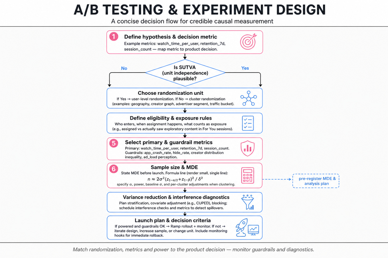
These interviews test whether a Data Scientist can design a credible causal measurement plan when naive user-level randomization is not enough. TikTok cares because recommendation, ads, notifications, and creator ecosystems have strong network effects, seasonality, and feedback loops: one user’s treatment can change another user’s feed, advertiser auction pressure, or creator supply. The interviewer is probing for disciplined thinking around randomization units, metric hierarchy, power, variance reduction, interference diagnostics, and launch decisions under uncertainty. Strong answers sound like an experiment plan a product team could actually run, not a generic “split users 50/50 and compare means.”

Core knowledge

• Unit of randomization is the first design choice, not an implementation detail. User-level randomization works when outcomes are independent; switch to cluster randomization by geography, creator graph, advertiser segment, or traffic bucket when spillovers violate SUTVA: “one unit’s outcome is unaffected by another unit’s treatment.”

• Eligibility and exposure rules prevent diluted or biased effects. Define who can enter the experiment, when assignment occurs, and what counts as treatment exposure. For a recommendation experiment, distinguish assigned users from users who actually saw exploratory content in For You sessions.

• Primary metrics should map to the decision being made. For recommendations, use metrics like watch_time_per_user, retention_7d, session_count, like_rate, hide_rate, and content diversity. For monetization, separate user value metrics from business metrics such as revenue_per_mille, cost_per_conversion, or advertiser_ROAS.

• Guardrail metrics catch harmful regressions that the primary metric hides. Examples include app_crash_rate, report_rate, not_interested_rate, creator distribution inequality, ad load perception, 7d_retention, and latency-sensitive engagement. A lift in short-term watch_time may be unacceptable if hide_rate or churn increases.

• Sample size and MDE should be stated before launch. For a two-sample mean comparison, a common approximation is:
  $n \approx \frac{2\sigma^2(z_{1-\alpha/2}+z_{1-\beta})^2}{\delta^2}$
  where $\delta$ is the minimum detectable effect, $\sigma^2$ is outcome variance, $\alpha$ is false positive rate, and $1-\beta$ is power.

• Ratio metrics need care because the denominator is random. Metrics like cost_per_conversion = spend / conversions or watch_time_per_session are not simple averages. Use the delta method, bootstrap, or analyze numerator and denominator jointly to avoid misleading variance estimates.

• Variance reduction improves sensitivity without increasing traffic. CUPED adjusts outcomes using pre-experiment covariates:
  $Y_{adj}=Y-\theta(X-\bar X), \quad \theta=\frac{Cov(Y,X)}{Var(X)}$
  It works best when pre-period behavior strongly predicts post-period outcomes, such as historical watch_time predicting future engagement.

• Seasonality must be designed around, not hand-waved away. Run treatment and control concurrently, cover full weekly cycles, avoid major holidays or product launches when possible, and stratify or block by time zone, geography, device, and traffic source if those dimensions strongly affect baseline behavior.

• Interference and spillovers change the estimand. In creator or ads markets, treatment can affect inventory, competition, prices, and untreated users’ experiences. Decide whether you want a direct effect, total effect, or market-level effect; then choose user, cluster, geo, or switchback designs accordingly.

• Switchback experiments are useful when treatment affects a shared marketplace or ranking environment. Alternate treatment and control by time block or region, then compare outcomes with time fixed effects. They are common for ads auction changes, feed ranking systems, and supply-demand balancing, but are vulnerable to carryover effects.

• Sequential monitoring must control false positives. Repeatedly checking p < 0.05 inflates Type I error. Use pre-planned looks with alpha spending, group sequential tests, or Bayesian decision thresholds; otherwise, report results as exploratory rather than confirmatory.

• Observational causal inference is a fallback, not a free substitute for randomization. Use difference-in-differences, propensity score matching, inverse propensity weighting, or synthetic controls only after stating assumptions like parallel trends, overlap, and no unobserved confounding. Always include falsification checks and sensitivity analysis.

Tip: In an interview, structure your answer as: objective → hypothesis → unit and assignment → metrics → power → validity risks → analysis plan → decision rule.

Worked example

For Design robust A/B test with interference and seasonality, a strong candidate would start by clarifying the product surface, the expected mechanism, and whether users interact through shared content, creators, or ads inventory. In the first 30 seconds, they might say: “I’ll define the causal estimand, check whether user-level randomization is valid, then design randomization, metrics, power, and diagnostics around interference and seasonality.” The answer should first identify the treatment, eligible population, and exposure event, such as users who open For You during the experiment window. Second, define a metric hierarchy: primary engagement or retention metric, guardrails like hide_rate and report_rate, and ecosystem metrics such as creator exposure concentration. Third, choose the assignment design: if spillovers are weak, use stratified user-level randomization; if content supply or social graph effects are strong, use cluster or geo-level randomization. Fourth, handle seasonality by running concurrent control, covering at least one or two full weekly cycles, and adding fixed effects for day-of-week, region, or traffic source. A key tradeoff to flag is that cluster randomization reduces contamination but lowers power because effective sample size depends on intra-cluster correlation, often summarized by design effect $1+(m-1)\rho$. The close should be practical: “If I had more time, I’d add pre-period CUPED covariates, interference diagnostics comparing treated-neighbor exposure, and a pre-registered sequential monitoring plan.”

A second angle

For Design A/B Test for Cost-Per-Conversion Efficiency Analysis, the same discipline applies, but the metric and marketplace constraints are different. The core outcome is usually cost_per_conversion, a ratio metric where spend and conversions can move in opposite directions, so the analysis should inspect spend, impressions, clicks, conversions, and conversion_value separately. Randomization may need to happen at advertiser, campaign, or auction-traffic level to avoid contamination between treatment and control bidding strategies. The candidate should discuss multi-arm allocation, power for sparse conversion events, and heterogeneous effects by advertiser size or vertical. The main tradeoff is between a clean advertiser-level experiment with less contamination and an auction-level design with more power but higher risk of interference through price dynamics.

Common pitfalls

Pitfall: Treating interference as a footnote.

A tempting answer is “randomize users 50/50 and compare average watch_time.” That fails if treatment changes shared content distribution, creator incentives, ad auction prices, or recommendations seen by untreated users. A better answer states the SUTVA risk explicitly and proposes cluster, geo, or switchback designs when the product mechanism requires them.

Pitfall: Optimizing one metric without a decision framework.

Candidates often pick watch_time or revenue as the only success metric. TikTok-style experiments require a metric hierarchy: one primary decision metric, supporting diagnostics, and hard guardrails for user experience, creator health, advertiser value, or long-term retention. The launch recommendation should say what happens under mixed results, not just whether the primary metric is statistically significant.

Pitfall: Overusing advanced methods without explaining assumptions.

Dropping terms like CUPED, propensity scores, or difference-in-differences is not enough. For CUPED, explain that pre-period covariates must be unaffected by treatment; for difference-in-differences, explain parallel trends; for matching, explain overlap and unobserved confounding. Interviewers reward clear assumptions more than method name-dropping.

Connections

Interviewers may pivot from here into causal inference, metric design, ranking/recommender evaluation, power analysis, or long-term network effects. Be ready to connect online experiment results to offline model metrics like AUC, NDCG, calibration, or counterfactual policy evaluation, while keeping the final decision grounded in user and business outcomes.

Further reading

• Trustworthy Online Controlled Experiments — Kohavi, Tang, and Xu’s practical book on experiment design, metrics, pitfalls, and organizational decision-making.

• Improving the Sensitivity of Online Controlled Experiments by Utilizing Pre-Experiment Data — Deng, Xu, Kohavi, and Walker’s CUPED paper, useful for variance reduction discussions.

• Causal Inference for Statistics, Social, and Biomedical Sciences — Imbens and Rubin’s rigorous foundation for potential outcomes, matching, and observational causal inference.

Practice questions

Statistics & Math

What's being tested

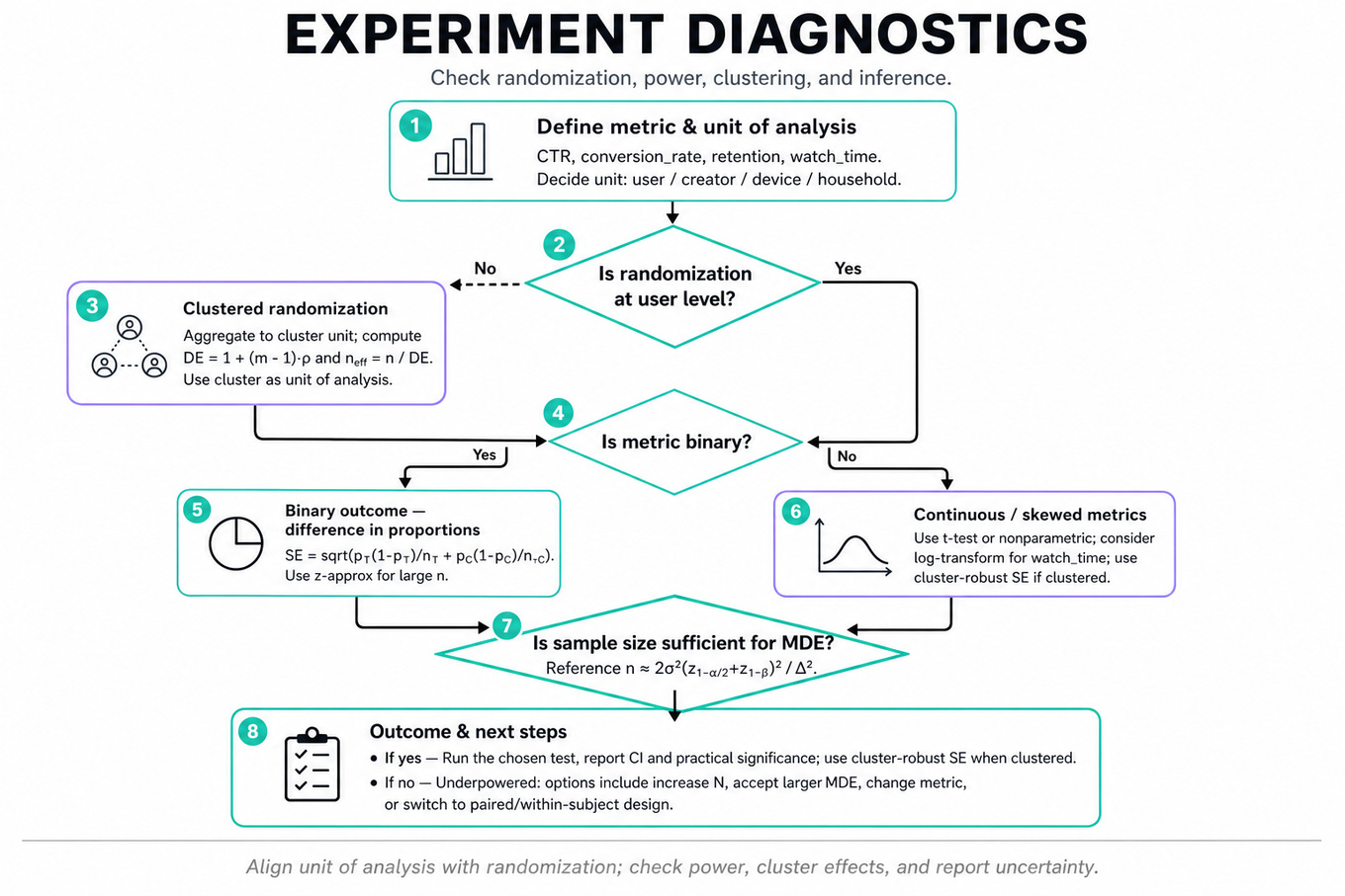
Interviewers are probing whether you can treat experiment results as statistical evidence, not just dashboard deltas. For a TikTok Data Scientist, this means diagnosing whether an observed change in CTR, conversion_rate, retention, watch_time, or posting behavior is causal, sufficiently powered, correctly randomized, and robust to known failure modes. You are expected to know when a simple two-sample test is valid, when clustered users or repeated looks break assumptions, and how to communicate uncertainty to product and engineering partners. The strongest answers combine inference, metric intuition, and practical experiment diagnostics.

Core knowledge

• Difference-in-proportions testing is the default for binary outcomes such as conversion, activation, or retention. For treatment rate $\hat p_T$ and control rate $\hat p_C$, use
  $SE=\sqrt{\frac{\hat p_T(1-\hat p_T)}{n_T}+\frac{\hat p_C(1-\hat p_C)}{n_C}}$
  and test $(\hat p_T-\hat p_C)/SE$ under large-sample normal approximation.

• One-sample proportion tests compare an observed rate $\hat p$ against a benchmark $p_0$, such as testing whether campaign conversion exceeds 60%. Use $SE=\sqrt{p_0(1-p_0)/n}$ for the null test, while confidence intervals often use $SE=\sqrt{\hat p(1-\hat p)/n}$ or Wilson intervals for better coverage.

• Power analysis asks whether the experiment could detect a practically meaningful effect. For a two-arm test, approximate required sample size per group scales as
  $n \approx \frac{2\sigma^2(z_{1-\alpha/2}+z_{1-\beta})^2}{\Delta^2}$
  so halving the minimum detectable effect requires roughly 4x more sample.

• Clustered randomization matters when assignment happens at creator, region, school, household, device group, or market level instead of user level. Observations inside a cluster are correlated, reducing independent information. Design effect is commonly approximated as $DE=1+(m-1)\rho$, where $m$ is average cluster size and $\rho$ is intra-cluster correlation.

• Effective sample size under clustering is roughly $n_{\text{eff}}=n/DE$. If 1M events come from highly correlated clusters, the inferential sample size may be closer to thousands of clusters than millions of rows. The unit of analysis should align with the unit of randomization.

• Cluster-robust standard errors estimate uncertainty while allowing arbitrary correlation within clusters. In practice, you can aggregate to cluster-level outcomes or use sandwich estimators, but you need enough clusters; with fewer than roughly 30–50 clusters, use caution, small-sample corrections, or randomization inference.

• Sequential testing handles repeated peeking at experiment results. If you check daily and stop when $p<0.05$, the false positive rate exceeds 5%. Use alpha-spending rules such as O’Brien-Fleming for conservative early looks or Pocock for more even thresholds across interim analyses.

• Sample ratio mismatch is a core randomization diagnostic. If the planned allocation is 50/50 but observed traffic is 53/47, test counts with a chi-square goodness-of-fit test before interpreting effects. SRM can indicate eligibility bugs, logging gaps, treatment leakage, or platform-specific exposure differences.

• Right-censoring appears in cohort behavior when some users have had less time to produce an outcome, such as 7-day posting after signup. Avoid comparing incomplete windows directly. Use fixed mature cohorts, survival analysis, or clearly defined observation windows such as posts_within_7d.

• Heavy-tailed metrics like watch_time, revenue_per_user, comments, shares, or posts per creator often violate normal assumptions at the user level. Robust choices include winsorization, log transforms, bootstrap confidence intervals, quantile metrics, or pre-registered capped means.

• Metric denominator discipline prevents misleading effects. conversion_rate can mean conversions per impression, per exposed user, per eligible user, or per session. Always identify numerator, denominator, eligibility, attribution window, and whether repeated exposures are counted.

• Heterogeneity and segmentation are diagnostic tools, not fishing licenses. Segment by pre-specified dimensions such as country, app version, traffic source, device, creator size, or new versus existing users. Use interaction tests or hierarchical thinking instead of declaring wins from noisy subgroup deltas.

Worked example

For “Diagnose Traffic Allocation in A/B Test Results”, a strong candidate would start by clarifying the intended randomization unit, planned split, exposure definition, eligibility rules, ramp schedule, and whether the metric is based on assigned users or actually exposed users. In the first 30 seconds, say: “Before estimating treatment impact, I’d verify randomization integrity and data consistency, because allocation bias can invalidate causal interpretation.”

The answer can be organized into four pillars: first, check sample ratio mismatch by comparing observed assignment counts to expected allocation using a chi-square test; second, inspect whether mismatch is concentrated by country, device_os, app_version, traffic source, or experiment ramp date; third, compare pre-treatment covariates and historical metrics across arms to detect imbalance; fourth, evaluate whether exposure, logging, or eligibility definitions create post-randomization filtering.

A good candidate would distinguish between assignment-based analysis and exposure-based analysis. Assignment-based intent-to-treat preserves randomization but may dilute effects if many assigned users were never exposed. Exposure-based analysis can answer a product adoption question but may be biased if exposure itself is affected by treatment or user behavior.

One explicit tradeoff to flag: pausing analysis to debug SRM protects causal validity, but if the experiment is on a critical launch path, you may provide clearly labeled descriptive readouts while withholding causal claims. The close should be pragmatic: “If I had more time, I’d audit pre-period balance, run the same diagnostics on guardrail metrics like crash_rate and session_starts, and compare results across mature cohorts before recommending launch or rollback.”

A second angle

For “Compute cluster-aware significance and sequential corrections”, the same diagnostic mindset applies, but the main threat is not just bad allocation; it is invalid uncertainty. If the experiment randomizes by market or creator cluster but the analyst tests millions of user rows as independent, the $p$-value will be artificially small. A strong answer identifies the randomization unit, estimates or reasons about the intra-cluster correlation, applies a design effect or cluster-robust standard error, and then adjusts thresholds for interim looks using an alpha-spending rule. The framing shifts from “is the treatment assignment trustworthy?” to “is the evidence calibrated after dependency and repeated monitoring?”

Common pitfalls

Pitfall: Treating row count as sample size when rows are correlated.

A tempting answer is: “We have 10 million events, so the test is highly powered.” That can be wrong if the experiment was randomized by 200 regions or creators, or if each user contributes many events. A better answer anchors inference to the randomization unit and discusses cluster-robust or user-level aggregation.

Pitfall: Reporting a significant lift before checking diagnostics.

Saying “treatment increased conversion_rate by 2%, $p<0.05$, ship it” is incomplete. Interviewers expect you to check SRM, pre-period balance, logging consistency, novelty effects, metric denominators, and guardrails before making a causal recommendation. The analytical maturity is in knowing when not to trust a clean-looking result.

Pitfall: Overcomplicating the answer without product interpretation.

A purely mathematical answer full of formulas but no decision framing can miss the Data Scientist role. For TikTok-style experiments, connect the inference back to launch decisions: expected user impact, risk to retention or watch_time, robustness across major segments, and whether the observed effect is practically meaningful, not merely statistically significant.

Connections

Interviewers may pivot from here into causal inference, especially intent-to-treat versus treatment-on-the-treated, CUPED variance reduction, difference-in-differences, or interference/network effects. They may also ask about metric design, cohort retention analysis, anomaly diagnosis after a release, or robust evaluation of recommender and ranking changes.

Further reading

• Trustworthy Online Controlled Experiments by Kohavi, Tang, and Xu — practical experimentation reference covering SRM, ramping, metrics, and common online testing traps.

• Group Sequential Methods with Applications to Clinical Trials by Jennison and Turnbull — rigorous treatment of sequential monitoring, alpha spending, and stopping boundaries such as O’Brien-Fleming.

• Mostly Harmless Econometrics by Angrist and Pischke — strong grounding for causal inference, clustered standard errors, and regression-based empirical reasoning.

Practice questions

What's being tested

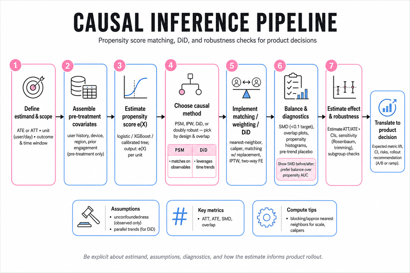
Interviewers are probing whether you can estimate causal impact when randomization is unavailable or imperfect, not just whether you can run a regression. For a TikTok Data Scientist, this matters because many product, ads, commerce, and notification decisions are made from logged observational data where exposed users differ systematically from unexposed users. You need to define the treatment, outcome, unit of analysis, and time window, then choose between methods like propensity score matching, inverse probability weighting, difference-in-differences, or doubly robust estimation. Strong answers show assumptions, diagnostics, sensitivity checks, and how the estimate would guide a product decision.

Core knowledge

• Causal estimands must be explicit: ATE estimates $E[Y(1)-Y(0)]$ for the whole population, while ATT estimates $E[Y(1)-Y(0)\mid T=1]$ for treated users. For TikTok product launches, ATT is often natural if asking “what happened to users who received the feature?”

• Potential outcomes frame the missing-data problem: each user has $Y_i(1)$ and $Y_i(0)$, but only one is observed. The causal effect is not simply $E[Y\mid T=1]-E[Y\mid T=0]$ unless treatment is independent of potential outcomes.

• Confounding occurs when pre-treatment variables affect both treatment and outcome. For example, heavy TikTok users may be more likely to receive notifications and also more likely to retain, inflating the apparent impact of notification exposure on D7_retention.

• Propensity score is $e(X)=P(T=1\mid X)$, usually estimated with logistic regression, XGBoost, or calibrated tree models. It reduces many covariates into one balancing score, but it only adjusts for observed pre-treatment covariates, not hidden motivation or intent.

• Matching pairs treated and control units with similar propensity scores or covariates. Common choices are nearest-neighbor matching, caliper matching, exact matching on key segments, and matching with replacement. For millions of users, exact pairwise matching can be expensive; use blocking, calipers, or approximate nearest neighbors.

• Balance diagnostics matter more than propensity model AUC. Check standardized mean differences before and after matching:
  $SMD = \frac{\bar X_T-\bar X_C}{\sqrt{(s_T^2+s_C^2)/2}}$
  A common target is absolute SMD < 0.1 for important covariates.

• Overlap, also called positivity, requires comparable treated and control users across the covariate space: $0 < P(T=1\mid X) < 1$. If high-value creators always receive a feature and low-activity users never do, causal effects are only credible within the overlapping segment.

• Difference-in-differences estimates treatment impact by comparing outcome changes over time:
  $\hat\tau = (\bar Y_{T,post}-\bar Y_{T,pre})-(\bar Y_{C,post}-\bar Y_{C,pre})$
  It is useful when treated and control groups differ in levels but would have followed parallel trends absent treatment.

• Parallel trends should be tested visually and quantitatively using multiple pre-periods. If treated users’ watch_time or repurchase_rate was already accelerating before exposure, a simple DiD estimate may attribute an existing trend to the intervention.

• Regression adjustment can complement matching or DiD. A typical DiD regression is $Y_{it}=\alpha_i+\gamma_t+\tau(T_i \times Post_t)+\epsilon_{it}$ with user and time fixed effects. Use clustered standard errors at the user, creator, market, or campaign level when outcomes are correlated.

• Doubly robust estimation combines propensity weighting with outcome modeling. Methods like AIPW remain consistent if either the propensity model or outcome model is correctly specified, making them attractive for observational ad lift or notification impact studies.

• Heterogeneous treatment effects ask who benefits, not just whether the average effect is positive. Use causal forests, meta-learners such as T-learners, S-learners, X-learners, or uplift models, but validate with honest sample splitting and avoid turning noisy subgroup effects into targeting policy.

Worked example

For Design causal measurement without randomization, a strong candidate would first clarify: “What exactly is the treatment: eligibility for the notification feature, actual notification sent, or notification opened?” They would also ask for the unit, likely user-level; the outcome, such as D7_retention; and the exposure and observation windows, such as feature exposure on day 0 and retention over days 1–7.

The answer skeleton should have four pillars. First, define a causal estimand, probably ATT: the impact on users who actually became eligible or received the notification. Second, draw the likely confounders: prior app opens, watch time, session frequency, country, device, tenure, notification settings, creator follows, historical retention, and prior push engagement. Third, propose a method: start with propensity score matching or inverse probability weighting using only pre-treatment covariates, then consider DiD if there are repeated pre/post outcomes. Fourth, discuss diagnostics: propensity overlap, covariate balance, placebo tests on pre-period outcomes, and sensitivity to calipers or model choice.

A specific tradeoff to flag is treatment definition. Estimating the effect of “notification opened” is more biased than estimating the effect of “notification sent” because openers are intrinsically more engaged; if logs support it, eligibility or send assignment is closer to an intervention. The candidate should close by saying that if more time were available, they would run robustness checks with doubly robust estimation, segment by new versus mature users, and compare the observational estimate to any future randomized holdout.

A second angle

For Analyze Negative Reviews' Impact on Coupon Repurchase Rate, the treatment is not a product exposure but an experience: receiving or seeing negative reviews before deciding whether to repurchase a coupon. The same causal machinery applies, but the confounding story changes: users who encounter negative reviews may be shopping different merchants, categories, price points, or deal types. A strong answer would define the unit as user-coupon or user-merchant, use pre-review covariates like historical purchase frequency, merchant rating, coupon discount, category, geo, and prior refund behavior, then estimate impact on coupon_repurchase_rate. DiD may be especially useful if the same merchants or cohorts can be observed before and after review shocks, but the candidate must check whether treated and comparison merchants had parallel repurchase trends before the negative reviews appeared.

Common pitfalls

Pitfall: Treating observational comparison as an A/B test.

A weak answer says, “Compare retention for users who got the feature versus users who did not.” That ignores selection bias. A better answer states the causal assumption explicitly: after conditioning on pre-treatment covariates, treatment assignment is as-good-as-random, then validates that assumption through balance, overlap, placebo outcomes, and sensitivity checks.

Pitfall: Optimizing the propensity model for prediction instead of balance.

A high AUC propensity model may separate treated and control users so well that there is little overlap, making matching unreliable. The goal is not to predict treatment perfectly; it is to create comparable groups. Report standardized mean differences, propensity score distributions, matched sample size, and which population the final estimate applies to.

Pitfall: Communicating only the method, not the decision implication.

Interviewers do not want a lecture that ends with “I would use PSM.” They expect an interpretation like: “If the ATT is +1.2 percentage points in D7_retention, confidence interval excludes zero, balance is acceptable, and placebo tests pass, I would recommend rollout for overlapping user segments, but not extrapolate to users outside support.”

Connections

Interviewers may pivot from here to A/B testing, sample ratio mismatch, metric design, uplift modeling, or off-policy evaluation for ranking and notification policies. They may also ask how you would combine causal estimates with product constraints such as user fatigue, long-term retention, creator ecosystem effects, or fairness across markets.

Further reading

• Causal Inference: The Mixtape — Practical coverage of DiD, matching, fixed effects, and modern causal designs.

• Imbens and Rubin, Causal Inference for Statistics, Social, and Biomedical Sciences — Rigorous foundation for potential outcomes, propensity scores, and treatment effects.

• Athey and Imbens, “Recursive Partitioning for Heterogeneous Causal Effects” — Key reference for causal trees and heterogeneous treatment effect estimation.

Practice questions

Machine Learning

What's being tested

TikTok is probing whether you can reason about recommender and ads objectives as measurable, causal, multi-sided optimization problems rather than as “maximize clicks.” A strong Data Scientist should translate business goals like user growth, creator monetization, ad revenue, and content diversity into ranking metrics, experiment designs, and trade-off analyses. Interviewers are looking for comfort with marketplace constraints: users, creators, advertisers, and platform health can have conflicting incentives. You should be able to define objective functions, diagnose metric movement, design A/B tests, and explain when an apparent offline model gain may not translate into product value.

Core knowledge

• Multi-objective ranking usually combines predicted outcomes into a scalar utility, for example:
  $score_i = w_1 \cdot P(watch)_i + w_2 \cdot E[watch\_time]_i + w_3 \cdot P(follow)_i - w_4 \cdot P(hide)_i + w_5 \cdot ad\_value_i$
  The DS task is not just choosing weights, but estimating marginal impact on DAU, retention, revenue, creator outcomes, and user satisfaction.

• Marketplace objectives require thinking across at least three sides: users want relevant content, creators want reach and monetization, and advertisers want conversions at efficient cost. A ranking change that increases CTR can still harm creator diversity, ad load tolerance, or long-term retention.

• Ads ranking often uses expected value logic such as eCPM = bid × pCTR × pCVR × value_adjustment, with quality penalties or relevance constraints. For DS interviews, focus on metric design, calibration checks, auction outcome analysis, and experiment interpretation rather than low-level serving mechanics.

• Calibration matters because ranking scores are often used as probabilities or expected values. If predicted pCTR = 0.05, roughly 5% of comparable impressions should click. Poor calibration can over-allocate impressions to ads or content types with overconfident predictions, distorting both user experience and marketplace fairness.

• Diversity and novelty are not the same as relevance. Practical metrics include category entropy, creator exposure concentration, share of impressions from new creators, topic coverage, repeat-author rate, and Gini or HHI concentration over creators. A diversity intervention should be evaluated against guardrails like watch time, skips, hides, and retention.

• Long-term value is central in feeds. Short-term CTR, session length, or ad revenue may increase while D1/D7 retention or future session frequency falls. A common framing is estimating incremental lifetime value:
  $LTV = \sum_{t=0}^{T} \gamma^t \cdot E[value_t]$
  where value can include engagement, revenue, or creator ecosystem health.

• A/B testing should separate primary, secondary, and guardrail metrics. For a homepage carousel, primary metrics might be CTR or downstream watch time per exposed user; guardrails might be bounce_rate, hide_rate, session_duration, D7_retention, and ad revenue per mille. Avoid declaring success from one favorable metric if key guardrails regress.

• Power and minimum detectable effect matter because recommender changes often create small lifts. A rough two-sample proportion test uses
  $n \approx \frac{2(z_{\alpha/2}+z_\beta)^2 p(1-p)}{\delta^2}$
  per arm. For rare events like purchases or advertiser conversions, use longer experiments, variance reduction, triggered analysis, or aggregate marketplace metrics.

• Triggered analysis is often more appropriate than all-user analysis. If only users who see a carousel or ad slot can be affected, estimate treatment effects on the exposed population, while also tracking ecosystem-level metrics across all users to catch spillovers.

• Causal inference is needed when experiments are unavailable or contaminated. Useful tools include difference-in-differences, propensity score weighting, synthetic controls, and instrumental variables, but you must state assumptions. For ranking systems, selection bias is severe because shown items are not random samples of all eligible items.

• Interference and network effects are common. A creator whose impressions increase in treatment may lose impressions in control-like contexts, and ads auctions can shift prices across advertisers. If interference is likely, consider cluster randomization by geography, user, advertiser, or creator cohort, depending on the treatment.

• Segmentation is essential but dangerous. Always inspect effects by new vs. returning users, heavy vs. light users, creator size, content category, advertiser vertical, and market. If testing dozens of segments, control false positives with methods like Benjamini-Hochberg FDR rather than cherry-picking the best-looking slice.

Worked example

For Design recommendations objective balancing growth and monetization, a strong first 30 seconds would clarify whether “growth” means DAU, new-user activation, retention, total watch time, or session frequency, and whether “monetization” refers to ad revenue, creator earnings, in-app purchases, or advertiser ROI. I would state an assumption: we are ranking organic and monetizable inventory in a feed-like surface, and the goal is to improve long-term platform value without degrading user trust.

The answer can be organized into four pillars. First, define a north-star objective such as incremental long-term value per user, with components for engagement, retention, revenue, and negative feedback. Second, propose a ranking utility function that combines predicted organic engagement, ad value, creator value, and penalties for low-quality experiences. Third, design an experiment framework with primary metrics like D7_retention or session frequency, monetization metrics like ARPDAU and ad eCPM, and guardrails like hide_rate, report_rate, and creator exposure concentration. Fourth, explain a trade-off policy, such as maximizing revenue subject to no statistically significant decline in retention or keeping ad load within user-tolerance bands.

One explicit design decision is whether to use a weighted objective or a constrained objective. A weighted score is easier to tune, but constraints are clearer for marketplace trust: for example, “increase ARPDAU only if D7_retention does not fall by more than 0.1 percentage points and advertiser CPA does not worsen.” I would close by saying that if I had more time, I would estimate heterogeneous treatment effects by user maturity, creator tier, and advertiser vertical, because a global average can hide harmful reallocations.

A second angle

For Improve TikTok's Algorithm for Diverse Content Discovery, the same concept shifts from monetization trade-offs to relevance versus exploration. The candidate still needs to define a utility function, but now it may include novelty, topic coverage, creator diversity, and long-term satisfaction rather than ad value. The experiment design should guard against “fake diversity,” where the feed shows more categories but users skip more, hide more, or return less often. A good answer would compare approaches like entropy-based re-ranking, maximal marginal relevance, creator exposure caps, or exploration buckets, while emphasizing measurement: diversity is only valuable if it improves discovery, retention, or creator ecosystem health. The core transfer is that ranking objectives must be evaluated causally and multi-dimensionally, not optimized against one offline metric.

Common pitfalls

Pitfall: Treating CTR or watch time as the whole objective.

This is the classic analytical mistake. Maximizing clicks can reward clickbait, repetitive content, low-quality ads, or addictive short sessions that hurt D7_retention. A better answer distinguishes immediate engagement, long-term satisfaction, monetization, advertiser value, and ecosystem health.

Pitfall: Giving a product slogan instead of a measurable decision rule.

Saying “we should balance users and advertisers” is not enough. Translate balance into constraints, weights, or launch criteria: for example, “ship if ARPDAU increases by at least 1%, D7_retention is non-inferior within 0.1 pp, and hide_rate does not increase for new users.”

Pitfall: Ignoring selection bias in recommender evaluation.

Offline comparisons of clicked versus unclicked items are biased because users only interact with what the current system chose to show. Stronger answers mention randomized buckets, exploration traffic, counterfactual evaluation, inverse propensity weighting, or at minimum why offline AUC is insufficient for launch decisions.

Connections

Interviewers may pivot from this topic into A/B testing, causal inference, metric design, uplift modeling, or fairness in marketplace allocation. They may also ask how to diagnose metric regressions by cohort, how to handle novelty effects, or how to evaluate recommender quality when long-term outcomes take weeks to observe.

Further reading

• Recommender Systems Handbook, Ricci, Rokach, and Shapira — broad foundation on ranking, diversity, evaluation, and recommender trade-offs.

• Practical Lessons from Predicting Clicks on Ads at Facebook — useful for understanding ads prediction, calibration, and large-scale ranking evaluation from a metrics lens.

• Hidden Technical Debt in Machine Learning Systems — helpful context for why offline model gains can create unexpected production and measurement issues.

Practice questions

What's being tested

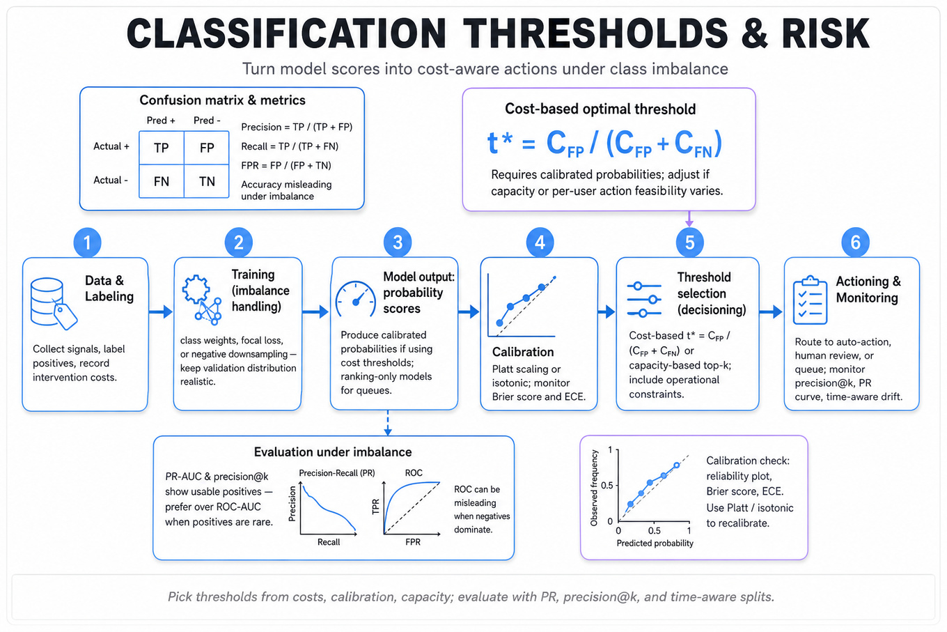
Interviewers are probing whether you can turn a probabilistic classifier into a risk-aware decision system, especially when positives are rare and mistakes have asymmetric costs. For a Data Scientist at TikTok, this matters in settings like fraud, spam, policy-risk detection, creator churn, user retention, and ads quality, where a model score is not the same thing as an action. Strong answers show fluency in class imbalance, threshold selection, cost-sensitive evaluation, calibration, and time-aware validation. The interviewer is not just asking “which model performs best,” but whether you can define the right objective, diagnose failure modes, and recommend a threshold that matches product constraints.

Core knowledge

• Classification thresholds convert predicted probabilities or scores into actions: predict positive if $\hat{p}(y=1 \mid x) \ge t$. The optimal threshold is rarely 0.5; it depends on base rate, intervention capacity, user harm, false-positive cost, false-negative cost, and downstream action quality.

• Confusion matrix metrics are threshold-dependent: precision $= TP/(TP+FP)$, recall $= TP/(TP+FN)$, FPR $= FP/(FP+TN)$, and FNR $= FN/(FN+TP)$. In imbalanced problems, accuracy is usually misleading because predicting the majority class can look excellent.

• Expected cost minimization gives a principled threshold when costs are known. If false positive cost is $C_{FP}$ and false negative cost is $C_{FN}$, classify positive when $C_{FP}(1-p) < C_{FN}p$, implying $t^* = \frac{C_{FP}}{C_{FP}+C_{FN}}.$ This assumes calibrated probabilities and equal action feasibility across users.

• Precision-recall curves are often more informative than ROC-AUC under severe imbalance. ROC-AUC can look high when negatives dominate, while PR-AUC and precision at operational recall reveal whether positive predictions are usable for real intervention queues.

• Calibration means predicted probabilities match empirical frequencies: among users scored 0.8, about 80% should be positive. Use reliability plots, Brier score, expected calibration error, Platt scaling, or isotonic regression. Threshold policies based on costs require calibrated probabilities; ranking-only models need not be perfectly calibrated.

• Class imbalance handling should be separated into training, evaluation, and decisioning. Techniques include class weights, focal loss, downsampling negatives, oversampling positives, SMOTE, balanced bagging, and threshold tuning. Always evaluate on the natural population distribution unless the production population is intentionally reweighted.

• Bagging versus boosting differs under imbalance. Bagging methods like RandomForest reduce variance and can use balanced bootstrap samples; boosting methods like XGBoost, LightGBM, or CatBoost often perform well with scale_pos_weight, custom loss, and careful early stopping. Boosting can over-focus on mislabeled rare positives if labels are noisy.

• Time-aware validation is critical for fraud and churn. Random splits leak future behavior into training and overstate performance. Prefer train-on-past, validate-on-future splits, rolling windows, cohort-based evaluation, and monitoring performance by event time because fraud patterns, seasonality, and user lifecycle dynamics drift.

• Operational constraints often define the threshold. If a human review team can handle 10,000 cases/day, choose the threshold that yields the top 10,000 highest-risk cases and report expected precision/recall at that capacity. If user friction is costly, enforce a maximum FPR or maximum number of false blocks.

• Segment-level thresholds may be better than one global threshold when base rates and costs differ by country, device type, payment method, creator cohort, tenure, or traffic source. But segment thresholds can create fairness and stability risks, so compare segment-level FPR, FNR, calibration, and sample sizes before deployment.

• Business metrics should connect model performance to outcomes. For churn, a false positive may waste an incentive; a false negative may lose a high-LTV user. For fraud, a false positive may block a legitimate transaction; a false negative may cause chargeback loss. Translate TP, FP, FN into expected dollars, user trust, moderation load, or retention lift.

• Thresholds decay over time as base rates and score distributions shift. Monitor population score distribution, positive rate, precision on delayed labels, calibration drift, and segment-level lift. A fixed threshold can silently become too aggressive or too lenient after product changes, adversarial adaptation, or seasonal behavior shifts.

Worked example

For “How do you choose a classification threshold?”, a strong candidate would first ask: what action follows a positive prediction, what are the costs of false positives and false negatives, are probabilities calibrated, and is there a capacity constraint? They would state that threshold choice is a decision problem, not just a modeling problem, and that 0.5 is only reasonable under symmetric costs and calibrated probabilities. The answer can be organized around four pillars: define the objective, evaluate threshold-dependent metrics, incorporate business or operational constraints, and validate stability over time and segments.

A good skeleton answer might start with a validation set representing the real production distribution, then sweep thresholds and compute precision, recall, FPR, FNR, PR-AUC, expected cost, and action volume. If costs are known, choose the threshold minimizing expected cost; if capacity is fixed, choose the threshold that fills the intervention queue while maximizing expected value. The candidate should explicitly flag calibration: if scores are uncalibrated, the threshold can still rank users, but cost-based probability cutoffs are not trustworthy. One tradeoff to call out is whether to prioritize high precision to avoid harming legitimate users or high recall to catch more risky cases. A strong close would be: “If I had more time, I’d test threshold stability by week and segment, evaluate delayed labels, and run an online experiment to measure whether the intervention actually improves the downstream product metric.”

A second angle

For “Compare bagging vs boosting on imbalanced data,” the same concept appears through model selection rather than final decisioning. The candidate should explain that imbalance affects the learner’s loss function, the evaluation metric, and the threshold, so comparing RandomForest against XGBoost using only accuracy would be weak. Bagging with balanced samples can be robust and less sensitive to label noise, while boosting often achieves stronger ranking performance but may overfit rare noisy positives without regularization, time-aware validation, and class weighting. The threshold still must be tuned after model training because a boosted model with better ROC-AUC may not produce better precision at the actual review capacity. The framing shifts from “which cutoff should I use?” to “which model gives the best calibrated or ranked scores for the operating region I care about?”

Common pitfalls

Pitfall: Optimizing for accuracy on a rare-event problem.

If fraud rate is 0.2%, a model that predicts “not fraud” for everyone gets 99.8% accuracy and is useless. A stronger answer says to evaluate PR-AUC, precision at top K, recall at fixed FPR, cost-weighted loss, and expected business impact under the real base rate.

Pitfall: Treating model score, probability, and decision as the same thing.

Many candidates say “I’ll use 0.5” or “I’ll pick the highest F1” without explaining whether scores are calibrated or what action follows. Better: separate ranking quality, probability calibration, and threshold/action policy; then choose the threshold using costs, constraints, or experimental evidence.

Pitfall: Ignoring time and delayed labels.

Fraud, churn, and retention labels often arrive late, and behavior changes over time. A random train/test split can leak future information and inflate performance; a stronger candidate uses forward-looking validation, cohort cuts, delayed-label awareness, and monitors performance drift by week and segment.

Connections

Interviewers may pivot from thresholding into model calibration, uplift modeling, causal measurement of interventions, ranking metrics, or online experiment design. For TikTok-style products, expect follow-ups on segment analysis, fairness of false positives, delayed feedback loops, and how offline model metrics connect to online product metrics like retention, trust, moderation quality, or revenue.

Further reading

• “The Relationship Between Precision-Recall and ROC Curves” by Davis and Goadrich — foundational explanation of why PR curves are often better for imbalanced classification.

• “Probability Calibration” in The Elements of Statistical Learning by Hastie, Tibshirani, and Friedman — useful background on probabilistic classifiers and calibration.

• “Learning from Imbalanced Data” by He and Garcia — classic survey covering sampling, cost-sensitive learning, and evaluation pitfalls.

Practice questions

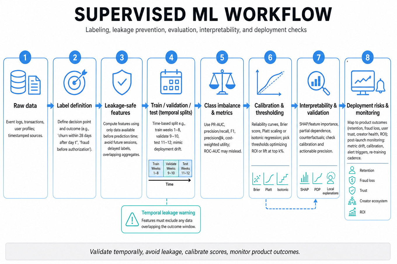
What's being tested

Interviewers are probing whether you can take a messy business prediction problem and turn it into a defensible supervised machine learning workflow: define the label, build leakage-safe features, choose evaluation metrics, interpret the model, and reason about deployment risks. At TikTok scale, a Data Scientist is expected to connect model quality to product outcomes such as retention, fraud loss, user trust, creator ecosystem health, and intervention ROI. The strongest answers show statistical discipline: temporal validation, class imbalance handling, calibration, threshold selection, and post-launch monitoring from a metric lens. You are not being tested on serving infrastructure internals; you are being tested on whether the model would be valid, useful, explainable, and measurable in production.

Core knowledge

• Problem framing starts with the prediction target, decision point, and action. For churn, define “churn within 28 days after day $t$”; for fraud, define whether a transaction is fraudulent based only on information available before authorization. A vague label creates noisy training data and misleading offline metrics.

• Temporal leakage is the most common supervised ML failure. Features must be computed using data available before the prediction timestamp. If predicting churn on Monday, do not include future sessions, future support tickets, delayed labels, or aggregates whose window overlaps the outcome period.

• Train/validation/test splits should mimic deployment. Prefer time-based validation over random splits for churn, fraud, ranking quality, and user behavior modeling because user behavior, abuse patterns, and product surfaces drift. A typical split is train on weeks 1–8, validate on weeks 9–10, test on weeks 11–12.

• Class imbalance changes metric choice and thresholding. For rare fraud or churn, accuracy can be meaningless. Use precision, recall, F1, PR-AUC, lift at top $k$%, and cost-weighted utility. ROC-AUC can look strong even when precision at actionable thresholds is poor.

• Calibration matters when scores drive decisions. If a model says a user has 0.8 churn risk, roughly 80% of similar users should churn. Use reliability curves, Brier score, Platt scaling, or isotonic regression. Calibration is especially important when ranking users for retention offers or fraud review queues.

• Threshold selection should optimize the business decision, not just a statistical metric. For binary classification, choose threshold $\tau$ using expected utility:
  $\text{Expected value} = TP \cdot B_{TP} - FP \cdot C_{FP} - FN \cdot C_{FN}$
  For churn, false positives may waste incentives; for fraud, false negatives may create direct loss.

• Feature engineering should reflect behavior and recency. Strong churn features include sessions in last 1/7/28 days, change in watch time, creator interactions, notification opens, failed payments, customer support contacts, and tenure. Use rolling windows, ratios, deltas, and cohort-normalized features rather than only lifetime totals.

• Baseline models are part of a strong answer. Start with logistic regression for interpretability and calibration, then compare against tree-based models such as XGBoost, LightGBM, or random forests. Deep models may help with high-dimensional behavior sequences, but interview answers should justify complexity with measurable lift.

• Model evaluation should include segment-level performance. Report metrics overall and by country, device type, new vs tenured users, creator vs viewer, payment tier, or traffic source. A model with strong global PR-AUC can still underperform or create unfair treatment in important cohorts.

• Interpretability requires matching the tool to the question. VIF diagnoses multicollinearity among predictors, often using $VIF_j = \frac{1}{1 - R_j^2}$. SHAP explains model predictions by attributing contribution to features. Under collinearity, SHAP credit can be split or unstable across near-duplicate features, while VIF flags the redundancy directly.

• Deployment readiness for a Data Scientist means defining acceptance criteria, guardrail metrics, and monitoring plans. Track prediction distribution, feature missingness, calibration drift, precision/recall on delayed labels, intervention take rate, and downstream product metrics such as DAU, retention, fraud loss, appeal rate, or user complaints.

• Unsupervised methods can support supervised workflows but rarely replace them when labels exist. K-means can segment users or initialize anomaly groups, using Lloyd’s iterations to minimize within-cluster SSE:
  $\sum_{i=1}^{n} \lVert x_i - \mu_{c_i} \rVert^2$
  But clusters need interpretation, stability checks, and validation against business outcomes.

Worked example

For Predict Customer Churn with Machine Learning Workflow, a strong candidate would first clarify: “What counts as churn, when is the prediction made, and what action will the business take?” They might assume the task is to predict whether an active user on day $t$ will be inactive for the next 28 days, using only data up to day $t$, so the model can trigger a retention intervention. The answer should be organized around four pillars: label definition, leakage-safe feature construction, model/evaluation strategy, and deployment measurement.

For features, they would propose recency/frequency/monetization-style behavior: sessions in the last 1/7/28 days, watch-time deltas, content diversity, notification engagement, social interactions, payment failures, tenure, and prior retention offer exposure. For modeling, they might start with logistic regression as a calibrated baseline, then compare LightGBM or XGBoost for nonlinear interactions. For evaluation, they should avoid accuracy and instead use PR-AUC, recall at fixed precision, lift in the top decile, calibration curves, and segment-level performance.

A specific tradeoff to flag is recall versus intervention cost: a low threshold catches more likely churners but may waste discounts or annoy users who would have stayed anyway. A polished answer closes by saying: “If I had more time, I would run an A/B test on the intervention policy, not just the model score, because the business goal is incremental retention, not offline AUC.”

A second angle

For Explain SHAP vs VIF under collinearity, the same workflow discipline appears in the interpretability and validation stage rather than model building. If two predictors are near duplicates, such as “sessions last 7 days” and “active days last 7 days,” VIF may be high because one feature can be linearly predicted from the other. SHAP may still generate attributions, but the credit assignment can be unstable: contribution may shift between correlated features depending on background data, model structure, or retraining sample. A strong Data Scientist would say VIF answers “are my predictors redundant or coefficients unstable?” while SHAP answers “what drove this model prediction?” They would recommend grouping correlated features, testing attribution stability, and validating whether removing one duplicate changes performance or interpretation.

Common pitfalls

Pitfall: Optimizing for accuracy on an imbalanced classification problem.

In churn or fraud, a model that predicts “not churn” or “not fraud” for everyone can have high accuracy and zero business value. A better answer names PR-AUC, precision at top $k$, recall at fixed false-positive rate, expected cost, and calibration.

Pitfall: Describing deployment as “put the model in production” without measurement.

For a Data Scientist, deployment readiness means defining launch criteria and monitoring metrics: score distribution drift, feature missingness, delayed-label performance, calibration, affected-user volume, and business impact through an experiment or holdout. Avoid going deep into infrastructure mechanics unless asked.

Pitfall: Treating interpretability tools as interchangeable.

Saying “SHAP tells us multicollinearity, so we do not need VIF” is wrong. VIF diagnoses predictor redundancy in the design matrix; SHAP explains model output contributions and can become ambiguous under correlated features. The stronger answer explains what each tool can and cannot claim.

Connections

Interviewers may pivot from this topic into causal inference, especially whether a churn intervention actually caused retention lift versus merely targeting users who would have stayed. They may also ask about A/B testing, ranking metrics, model calibration, fairness across cohorts, or anomaly diagnosis when offline and online metrics diverge.

Further reading

• Interpretable Machine Learning — Christoph Molnar — practical coverage of SHAP, feature importance, partial dependence, and interpretability caveats.

• The Elements of Statistical Learning — Hastie, Tibshirani, Friedman — rigorous treatment of supervised learning, regularization, classification, trees, and model assessment.

• Lundberg and Lee, “A Unified Approach to Interpreting Model Predictions,” NeurIPS 2017 — the original SHAP paper and useful background for attribution discussions.

Practice questions

Behavioral & Leadership

What's being tested

TikTok is probing whether a Data Scientist can turn ambiguous, high-stakes disagreement into a metric-grounded decision without losing stakeholder trust. Strong answers combine communication, experimental rigor, causal reasoning, and cross-functional leadership: you must explain what you know, what you do not know, and what evidence would change the decision. For a Data Scientist, this matters because product, engineering, policy, and compliance teams may optimize for different outcomes: growth, latency, creator fairness, user safety, monetization, or regulatory risk. Interviewers are looking for candidates who can lead through influence, not authority, while keeping decisions anchored to valid measurement rather than opinion.

Core knowledge

• Stakeholder alignment starts by separating goals, constraints, and fears. Product may care about `DAU`, `watch_time`, or creator supply; engineering may care about complexity and launch risk; policy or compliance may care about safety, privacy, or auditability. A strong DS translates these into measurable decision criteria.

• Metric hierarchy is the backbone of credible communication. Define a primary metric, supporting diagnostics, and guardrails: for example, primary `watch_time_per_user`, diagnostics like session depth and video completion rate, and guardrails like `report_rate`, `hide_rate`, creator distribution, or teen-safety metrics.

• Causal evidence beats descriptive lift when stakeholders are skeptical. A/B tests estimate $ATE = E[Y(1) - Y(0)]$ under randomization, while observational analyses need assumptions such as conditional exchangeability. If randomization is impossible, discuss difference-in-differences, propensity score weighting, or synthetic controls with explicit caveats.

• Experiment design should be explained in business language. Cover treatment, control, randomization unit, exposure definition, sample size, duration, novelty effects, and interference. In social or recommender systems, user-level randomization can create spillovers; creator-side or cluster randomization may be needed when treatment affects content supply.

• Statistical significance is not the same as decision significance. Report confidence intervals, effect size, and practical impact: “+0.3% `watch_time` with 95% CI [+0.1%, +0.5%], no movement in `report_rate`, equivalent to X incremental hours/day.” Avoid presenting only a `p_value`.

• Power analysis helps negotiate timelines. A simple minimum detectable effect approximation is $n \approx \frac{2(z_{1-\alpha/2}+z_{1-\beta})^2\sigma^2}{\Delta^2}$ for two equally sized groups. If stakeholders demand faster answers, offer tradeoffs: larger MDE, directional read, sequential testing, or narrower target cohort.

• Guardrail metrics prevent local optimization. A ranking change that improves `CTR` can harm long-term satisfaction if it increases clickbait, skips, negative feedback, or creator concentration. For TikTok-style feeds, credible DS answers balance short-term engagement with retention, user safety, content diversity, and ecosystem health.

• Segmentation is essential but dangerous. Break down effects by geography, device, new vs. existing users, creator size, content category, and sensitive policy-relevant cohorts where appropriate. But avoid cherry-picking; use pre-registered segments, interaction tests, or multiple-testing corrections such as Bonferroni correction or Benjamini-Hochberg FDR.

• Root-cause diagnosis should follow a metric tree. If `watch_time` drops, decompose into active users, sessions/user, videos/session, average watch duration, completion rate, and negative feedback. Then connect metric movement to product mechanisms instead of jumping to “the model got worse.”

• Conflict handling requires explicit decision rules. Before analysis ends, align on what outcome triggers launch, rollback, iteration, or escalation. For example: launch if primary metric improves by at least +0.2%, no statistically significant harm to `report_rate`, and no adverse movement in key teen-safety segments.

• Executive communication should be layered. Start with the recommendation, then evidence, then risks, then next steps. A good one-page readout includes decision, confidence level, metric table, caveats, owner, timeline, and “what would change my mind.”

• Leadership without authority means creating the process others trust. The Data Scientist does not “win” by having the most technical argument; they win by making assumptions visible, inviting challenges, documenting tradeoffs, and ensuring each function sees its concern reflected in the analysis.

Tip: In behavioral answers, use a structure like Situation → Conflict → Analysis → Alignment → Decision → Result → Reflection, but make the “Analysis” section concrete enough to prove you are a Data Scientist, not just a coordinator.

Worked example

For “Align Conflicting Stakeholders for Successful Project Delivery,” a strong candidate would first frame the situation in the first 30 seconds: “I’d clarify the product goal, the conflicting stakeholder incentives, the launch deadline, and which risks were non-negotiable versus optimizable.” They might choose an example where product wanted to ship a recommendation change to improve `watch_time`, engineering was concerned about implementation complexity, and compliance or policy wanted stronger evidence that vulnerable user segments were not harmed. The answer should be organized around four pillars: first, mapping each stakeholder’s concern into measurable criteria; second, designing the analysis or experiment; third, creating a shared decision framework; fourth, communicating the recommendation and follow-through.

The candidate should say they established a primary metric, such as `watch_time_per_user`, plus guardrails like `not_interested_rate`, `report_rate`, retention, and segment-level safety checks. They would explain that they used an A/B test or quasi-experimental readout to distinguish true lift from noise, then translated results into business impact and risk: “The treatment improved the primary metric by +0.4%, but one region showed elevated negative feedback, so I recommended a staged rollout excluding that region while we investigated.” A key tradeoff to flag is speed versus confidence: waiting for full power gives cleaner inference, while a staged rollout may meet business timelines with monitored risk. The leadership component is that the Data Scientist did not merely present a dashboard; they facilitated agreement on what evidence was sufficient before everyone saw the result. A strong close would include impact, such as successful launch, avoided rollback, or changed roadmap priority, plus a lesson learned: “If I had more time, I would define guardrail thresholds earlier and document escalation rules before the experiment started.”

A second angle

For “Communicate technical impact under skeptical stakeholders,” the same leadership skill is applied under a different constraint: the audience doubts whether the Data Scientist analysis proves causality. The framing should shift from negotiation among competing priorities to building evidentiary trust. A strong candidate would acknowledge skepticism directly, explain why a naive before/after comparison could be biased by seasonality or traffic mix, and present stronger evidence from randomized exposure, holdout groups, or robustness checks. They should avoid overclaiming: “The experiment supports causal lift for exposed users over two weeks; it does not yet prove long-term retention gains.” The best answers make the technical method understandable without diluting it: “Randomization makes treatment and control comparable in expectation, so the observed difference is attributable to the change, within the confidence interval.”

Common pitfalls

Pitfall: Treating stakeholder disagreement as a personality issue instead of a measurement and incentives issue.

A weak answer says, “I convinced everyone by explaining the data clearly.” That skips the hard part: different teams can rationally value different risks. A better answer identifies each stakeholder’s objective, converts it into metrics or constraints, and creates a decision rule everyone can accept.

Pitfall: Claiming impact without causal support.

A tempting behavioral answer is, “After my analysis, revenue increased 5%, so my project had huge impact.” For a Data Scientist interview, that is not enough. Say whether impact came from an A/B test, rollout comparison, matched cohort, diff-in-diff, or another method, and state the main validity threats.

Pitfall: Staying too high-level and sounding like a project manager.

Communication matters, but the interviewer still expects Data Scientist depth. Include concrete metric names, experimental design choices, confidence intervals, segmentation, and guardrails. The best answers show you can lead the room because your analytical reasoning improves the decision quality.

Connections

Interviewers may pivot from this topic into experiment design, metric design, causal inference, ranking/recommender evaluation, or root-cause analysis. They may also test behavioral variants such as handling missed deadlines, giving feedback to a teammate, escalating risk, or communicating a negative result to executives.

Further reading

• [Trustworthy Online Controlled Experiments, Kohavi, Tang, and Xu] — Practical reference for A/B testing, guardrails, ramp decisions, and communicating experimental evidence.

• [Crucial Conversations, Patterson et al.] — Useful framework for high-stakes disagreement, especially when you need to preserve trust while challenging assumptions.

• [Causal Inference: The Mixtape, Scott Cunningham] — Accessible grounding for causal reasoning, diff-in-diff, matching, and common observational-analysis pitfalls.

Practice questions

Take-home Project

Data Manipulation (SQL/Python)

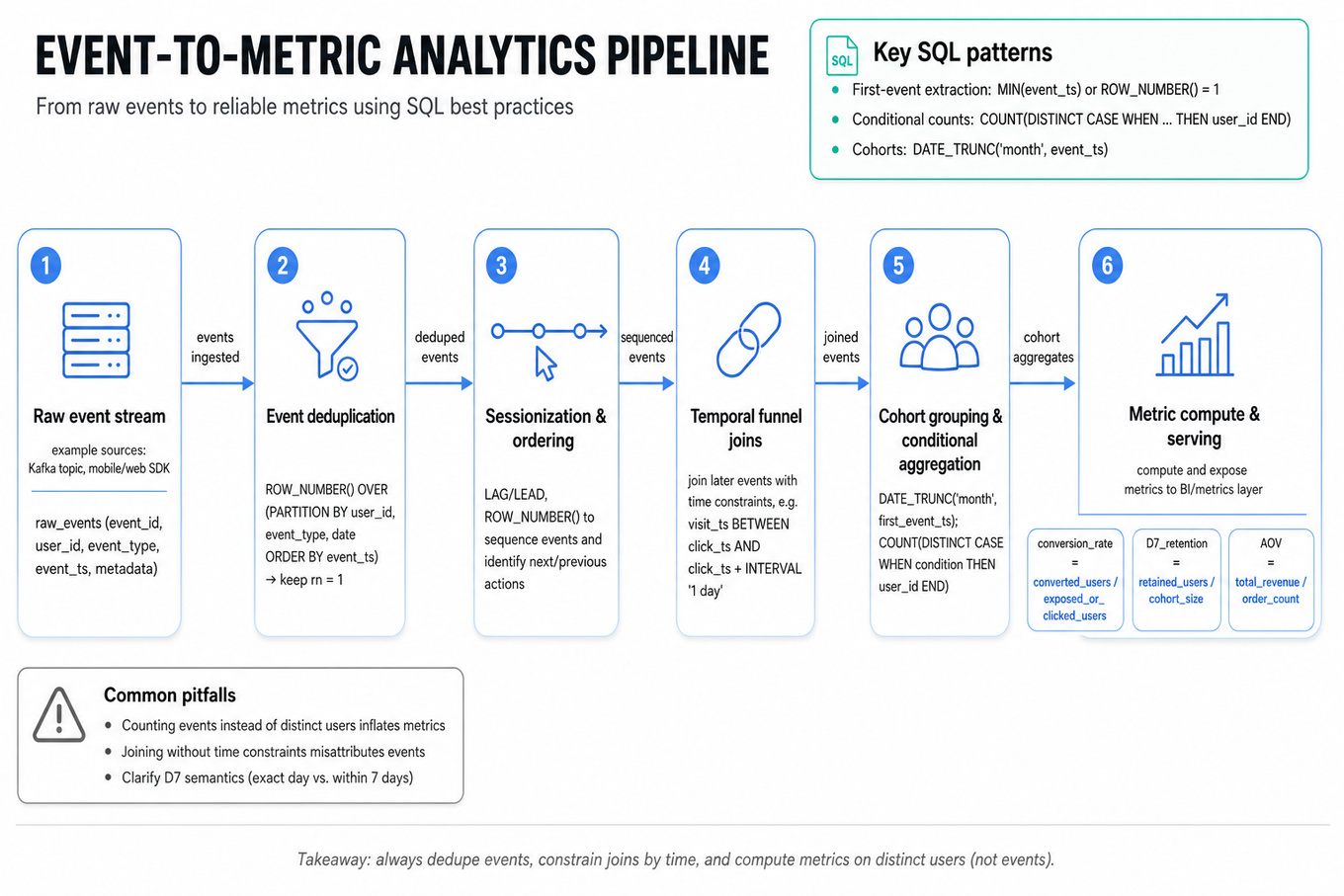
What's being tested

These prompts test analytical SQL for product metrics: deduplicating event streams, ordering user actions, joining behavioral tables, and computing cohort/funnel metrics. For a TikTok Data Scientist, the core skill is turning raw user events into trustworthy metrics like conversion_rate, D7_retention, AOV, and funnel step-through rates.

Patterns & templates

• Event deduplication with ROW_NUMBER() OVER (PARTITION BY user_id, event_type, date ORDER BY event_ts); keep rn = 1 before counting users.

• First-event extraction using MIN(event_ts) or ROW_NUMBER() to define registration date, first click, first visit, or cohort anchor.

• Temporal joins for funnels: join later events with conditions like visit_ts BETWEEN click_ts AND click_ts + INTERVAL '1 day'.

• Conditional aggregation with COUNT(DISTINCT CASE WHEN condition THEN user_id END) for conversion, retention, and step-level rates.

• Cohort grouping via DATE_TRUNC('month', event_ts) or registration date; compute rates as retained users divided by eligible cohort users.

• Window ordering with LAG, LEAD, and ROW_NUMBER to identify next action, prior action, session sequence, or valid event progression.

• Metric formulas should be explicit: conversion_rate = converted_users / exposed_or_clicked_users; AOV = total_revenue / order_count, not users.

Common pitfalls

Pitfall: Counting events instead of distinct users will inflate funnel conversion and retention when heavy users generate repeated actions.

Pitfall: Joining without time constraints can attribute a page visit, purchase, or post to the wrong prior event.

Pitfall: Using calendar day differences incorrectly; confirm whether D7 means exactly day 7, within 7 days, or days 1–7 after registration.

Practice these

The practice cards below cover the canonical variants — solve all of them and time yourself.

Practice questions