Analog Noise Budget Interview: Refer Sources to the Input and Integrate Bandwidth
Quick Overview
Build an analog noise budget with input-referred sources, source impedance, variance addition and integrated bandwidth using an original checked calculation. Primary references, original examples and explicit evidence limits support focused preparation.
To answer an analog noise-budget interview question, refer every source to the same point, combine uncorrelated contributions as noise power and integrate each source through its actual transfer function. The amplifier with the lowest voltage-noise density can lose when its current noise flows through a sufficiently large source impedance.
The original calculation below shows where the ranking reverses. For broader discussion practice, PracHub's thermal and signal fundamentals question is a useful starting point. Its scope is broader than this budget; the numerical exercise here supplies the input reference plane, bandwidth and assumptions needed for a checkable answer.
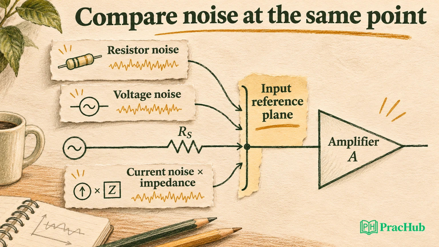
Primary manufacturer references establish the underlying mechanics. All component values, amplifier A/B specifications and computed results below are synthetic teaching inputs. No candidate report establishes a particular employer's question frequency, and no SPICE simulation, device characterization or silicon measurement is claimed.
Name the reference plane and the quantity
An input-referred noise budget expresses the output effects of different noise sources as equivalent noise at a chosen input. It lets you compare contributions that originated at different locations. State the reference plane and each source’s transfer. Otherwise comparable-looking numbers can describe different quantities.
Distinguish voltage-noise density, measured in volts per square root hertz, from integrated RMS voltage, measured in volts. Squaring an amplitude density gives a power spectral density in square volts per hertz. Integrating that density over frequency produces a variance; taking its square root produces RMS noise.
Analog Devices' AN-940 describes input voltage noise, input current noise and external contributions, including resistor thermal noise. It also explains why source impedance matters when comparing amplifiers. That is a manufacturer explanation of the model, not an endorsement of our fictional amplifier specifications. AN-940
For our first calculation, use one real source resistance feeding an ideal noiseless gain block, with all modeled noise referred to that input. The gain is ten and a common single-pole low-pass response follows it. We deliberately exclude feedback-network noise so the source-resistance trade-off remains visible; a complete circuit budget must add it.
Build the variance equation before entering numbers
Assume independent, flat sources and a real source resistance Rs. The input voltage-noise power density is the sum of the amplifier's voltage-noise density squared, its current-noise density squared times Rs squared, and the resistor's thermal-noise power density.
S_input = en² + (in × Rs)² + 4 k T Rs
input density = sqrt(S_input)
Here k is Boltzmann's constant and T is absolute temperature. The current-noise term becomes a voltage through the source impedance. If that impedance is frequency-dependent, replace the simple resistance factor with the appropriate magnitude-squared transfer rather than carrying a constant Rs through the entire calculation.
Do not add the three amplitude densities directly. With the independence assumption, variances add. Analog Devices' op-amp noise discussion explains this root-sum-square treatment and the distinction between internally generated random noise and interference arriving through the surrounding circuit. Op-amp noise
Independence is an assumption you must defend. Correlated sources require cross-spectral terms; two appearances of the same physical disturbance should not be counted as independent generators. A mains-frequency tone also needs different treatment from a flat random-noise density. State the model before using its arithmetic.
Compare two amplifiers at three source resistances
Our fictional amplifier A has voltage-noise density 2 nV/√Hz and current-noise density 2 pA/√Hz. Amplifier B has 6 nV/√Hz and 0.02 pA/√Hz. Keep both specifications flat across the modeled band and use 300 K for every resistor calculation.
At 100 Ω, current noise contributes only 0.2 nV/√Hz for A and 0.002 nV/√Hz for B. The resistor contributes about 1.287 nV/√Hz. A's smaller voltage-noise specification therefore wins in the total, rather than merely looking better on a headline datasheet number.
At 10 kΩ, A's current-noise contribution is 20 nV/√Hz, while B's is 0.2 nV/√Hz. The same source resistor contributes about 12.872 nV/√Hz to either choice. Now B's larger voltage-noise density is outweighed by its much smaller current-noise term.
| Source resistance | Resistor density | A total density | B total density | Lower modeled total |
|---|---|---|---|---|
| 100 Ω | 1.287 nV/√Hz | 2.387 nV/√Hz | 6.137 nV/√Hz | A |
| 10 kΩ | 12.872 nV/√Hz | 23.868 nV/√Hz | 14.203 nV/√Hz | B |
| 100 kΩ | 40.704 nV/√Hz | 204.110 nV/√Hz | 41.192 nV/√Hz | B |
The values come from the saved local calculation. They are not measurements or a comparison of named commercial parts. Changing temperature, impedance or frequency-dependent device noise can change both the totals and the ranking.
Solve the crossover and check what cancels
Set A's total variance equal to B's under the same source resistance and temperature. The resistor term is identical on both sides, so it cancels when finding which amplifier has lower total noise. It still contributes to the absolute budget and should not disappear from the final RMS result.
Rs² = (en_B² − en_A²) / (in_A² − in_B²)
Rs ≈ 2.83 kΩ
This crossover exists because A trades lower voltage noise for higher current noise. It is not a universal “optimal source resistance.” The signal source, input loading, bias-current error, available gain and other requirements may prevent choosing that resistance freely.
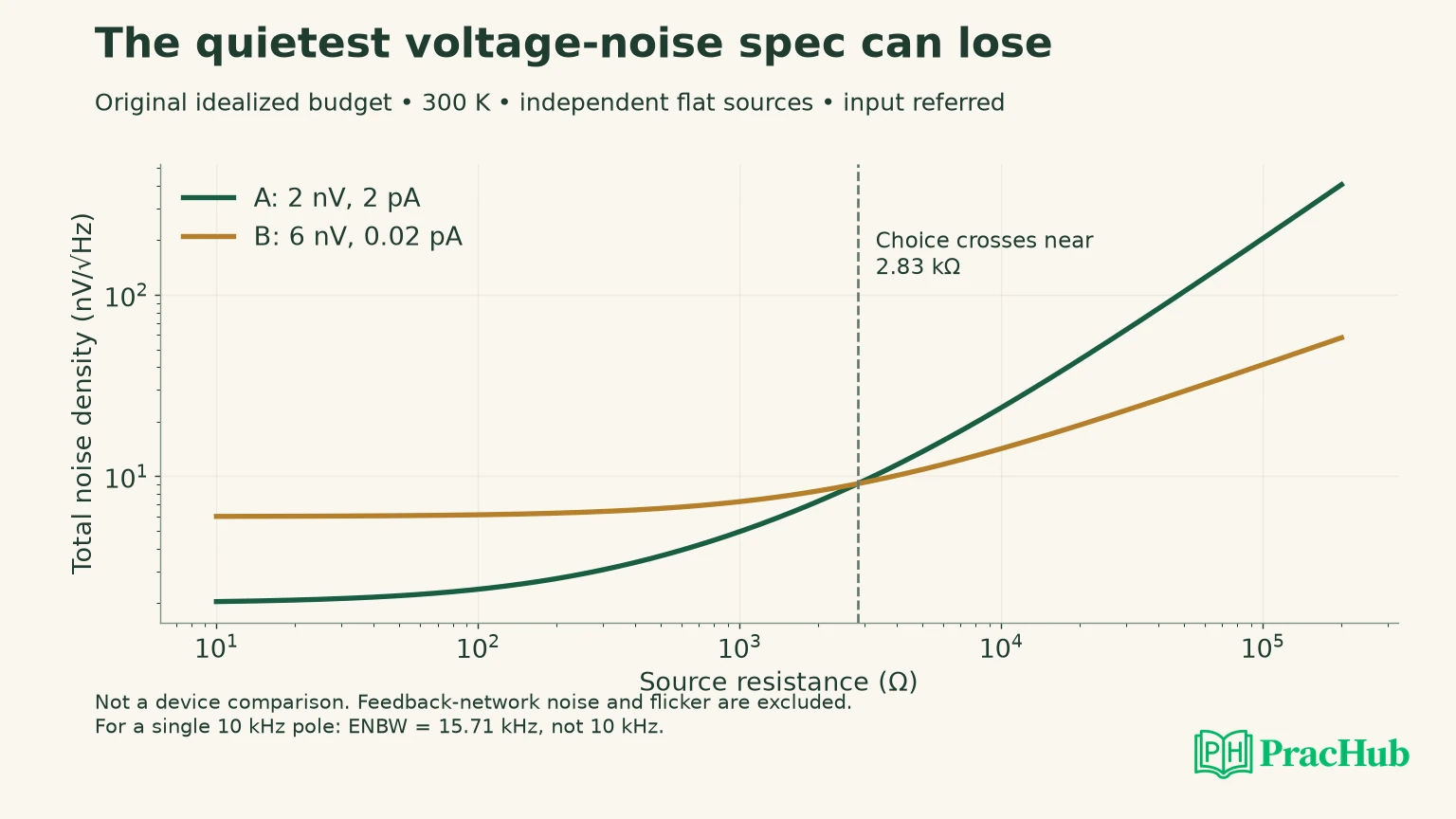
At high resistance, ask whether the resistor or amplifier current term dominates. Thermal amplitude density grows with the square root of resistance, while this flat current-noise voltage grows linearly with resistance. That difference explains the shape of the plotted curves and gives you a qualitative check before trusting the calculator.
A useful follow-up changes B's current noise by a factor of ten. Predict whether the crossover moves toward lower or higher resistance before recomputing it. You are testing the mechanism behind the ranking, rather than memorizing the original 2.83 kΩ result.
Integrate bandwidth rather than substituting the cutoff
A single-pole low-pass response does not remove all noise above its cutoff. For flat input noise and a response normalized to unity at DC, the equivalent noise bandwidth is the integral of the squared response. For the ideal single pole used here, it equals π/2 times the cutoff frequency.
With a 10 kHz cutoff, the equivalent noise bandwidth is therefore about 15.708 kHz. Multiplying density by the square root of 10 kHz would understate RMS noise. The correct RMS value is about 1.253 times that shortcut value for this particular model.
The manufacturer signal-chain guide defines equivalent noise bandwidth by equal integrated noise power and emphasizes declaring assumptions for each block. Its example is a different signal chain; our single-pole result follows from the stated transfer function. Signal-chain noise analysis
At Rs = 10 kΩ, A's input RMS noise is about 2.991 µV, while B's is 1.780 µV. With ideal signal gain ten and the common filter, the output values are about 29.914 µV and 17.800 µV. These numbers retain the same ranking because the two choices share the same modeled transfer.
Our Python/SciPy calculation independently integrated 1 / (1 + x²) from zero to infinity and compared it with π/2. That checks the numerical bandwidth calculation against an analytic result. It does not check whether a real amplifier has the assumed single-pole response or flat source densities.
Keep source-specific transfer functions separate
The common-filter simplification makes the worked budget compact. In a real circuit, noise injected after a filter does not pass through that earlier filter. Referring every source to the input does not authorize applying one bandwidth to sources that travel through different paths.
For a general budget, calculate each output contribution as the integral of its source power spectral density times its own transfer magnitude squared. Add the resulting variances, including correlation terms when needed. Only then convert the total to RMS or refer it back through a clearly defined signal gain.
Feedback resistors are a common missing contribution. Their thermal noise and the inverting-input current noise depend on the actual network. The amplifier's input voltage noise travels according to noise gain, which may differ from signal gain. Multiplying a headline density by signal gain can miss both circuit sources and their transfer functions.
Low-frequency flicker noise is another reason to name the integration limits. A white-noise model extending to DC does not represent every device's low-frequency spectrum. If the measurement removes DC or uses a finite observation window, describe that filtering explicitly rather than choosing a lower cutoff merely to obtain a smaller number.
Change the bandwidth without hiding the signal cost
For the same flat sources and filter shape, halving the cutoff halves noise variance and multiplies RMS noise by the square root of one half. The amplifier ranking stays unchanged in our common-transfer example. This is a calculation under the existing assumptions, not a new measurement.
Now ask whether the useful signal still passes. If the application needs to settle within a specified interval, a lower cutoff may violate that requirement. State the acceptable signal attenuation or settling error before proposing bandwidth reduction as the solution.
A second change halves amplifier A's voltage-noise density while leaving its current noise fixed. At 10 kΩ, the 20 nV/√Hz current contribution already dominates the 2 nV/√Hz voltage contribution. Reducing the smaller term cannot produce a proportionate reduction in total RMS noise. The variance equation tells you where a design change has limited benefit.
Use these counterfactuals as a sanity check on a spreadsheet. If halving a small contributor halves the total, inspect the summation and units before trusting the result. An independent qualitative prediction can catch a numerically tidy but incorrectly assembled budget.
Explain what the model does not diagnose
Suppose a bench trace contains occasional large spikes. Increasing a flat random-noise budget until it matches those spikes may conceal an interference or acquisition problem. Ask about grounding, supply coupling, sampling, probe bandwidth and the operating conditions before declaring that the amplifier's specified noise is wrong.
Likewise, a quieter output is not automatically a better signal chain. Excessive filtering may remove the signal or prevent required settling. Report the noise reduction together with the bandwidth and response-time cost. The relevant decision is whether the signal remains usable under the application's constraints.
For a proposed verification, name the measurement point, instrument noise floor, bandwidth and operating state. Explain how you would distinguish the circuit's contribution from the instrument's. Our calculated sweep is a prediction under assumptions; it should be compared with a suitably controlled measurement before becoming a device-performance claim.
Practice the calculation and the explanation
The first two PracHub records below address thermal or RF/analog fundamentals. The remaining records develop technical explanation and investigation. They do not constitute a dedicated five-question analog-noise bank, and none predicts a particular employer's interview.
| PracHub question | Rehearsal focus |
|---|---|
| Explain thermal and signal fundamentals | Use thermal and signal concepts to check units and reference points. |
| Explain RF/analog IC interview fundamentals | Connect source impedance and amplifier-noise terms; its broader RF scope differs. |
| Explain a Technical Project with an Architecture Diagram | Communication practice: show the measurement and system boundaries. |
| Explain Technology to a Nontechnical Audience | Communication practice: explain density versus RMS without unexplained jargon. |
| Demonstrate Project Ownership and In-Depth Investigation | Investigation practice: separate a noise hypothesis from the evidence that tests it. |
Use the thermal and signal question to rehearse the 10 kΩ case without the table. State the reference plane, calculate the three variance contributions and explain why B wins. Then change the cutoff and predict the RMS scaling before checking the integral.
Sources and Further Reading
- Analog Devices AN-940: amplifier selection and noise sources
- Analog Devices: op-amp noise, independence and source impedance
- Analog Devices: step-by-step signal-chain noise analysis
Sources checked November 3, 2026. All numerical results describe the original idealized budget, not measured hardware.
Comments (0)