Bandgap Reference Interview: Temperature Cancellation, Startup, and Trim
Quick Overview
Practice bandgap-reference interviews with PTAT and CTAT calculations, a startup review matrix and a trim example that exposes residual temperature errors. Primary references, original examples and explicit evidence limits support focused preparation.
A bandgap-reference interview answer should connect three separate questions: how temperature terms cancel, how the circuit reaches its intended operating point and what the available trim can correct. A correct nominal voltage does not establish reliable startup or low drift across temperature.
This article uses an original temperature model and a startup review matrix to keep those questions separate. PracHub's RF/analog IC fundamentals question provides broader analog discussion practice. The calculations below supply a focused bandgap exercise rather than a prediction of any employer's interview.

Manufacturer references establish the device principles. The coefficients, temperatures and computed outputs here are synthetic teaching inputs. We executed a local polynomial calculation, not a transistor-level SPICE simulation, startup transient or silicon characterization. No candidate-report set supports an employer-specific process claim.
Explain PTAT and CTAT before quoting a reference voltage
A bandgap reference combines a voltage with a negative temperature coefficient and a scaled voltage proportional to absolute temperature. In a common bipolar formulation, a base-emitter voltage supplies the complementary-to-absolute-temperature contribution, while the difference between two base-emitter voltages supplies a PTAT contribution.
Analog Devices' bandgap teaching activity describes combining these opposing terms. Its actual circuit also illustrates why output loading can disturb the intended relationship. The cancellation principle is not permission to ignore the surrounding bias, feedback and load circuitry. Bandgap reference activity
For the ideal relation used in this exercise, write ΔVBE = (kT/q) ln(N), where N represents the relevant current-density ratio. The ratio must follow from the chosen circuit's areas and currents. Do not automatically substitute an emitter-area ratio if the current assumptions do not support it.
The teaching expression is Vref = VBE + m × ΔVBE. Choosing m can cancel the local first derivative at a nominal temperature. It does not make every higher-order temperature term vanish, nor does it describe every modern reference architecture.
Calculate the scale factor with consistent units
Set the nominal temperature to 300 K, which is 26.85°C. Use N = 8, nominal VBE = 0.650 V and a local VBE slope of −1.8 mV/K. These are declared inputs for the exercise, not a specification for a named transistor or process.
At 300 K, kT/q is about 25.852 mV. Multiplying by ln(8) gives ΔVBE of about 53.758 mV. Its derivative with respect to temperature is approximately 0.1792 mV/K under the ideal fixed-ratio assumptions.
m = 1.8 mV/K ÷ [(k/q) ln(8)]
m ≈ 10.0451
m × ΔVBE at 300 K = 0.540 V
Vref at 300 K = 0.650 V + 0.540 V = 1.190 V
A common error is mixing millivolts with volts or Celsius with absolute temperature. The PTAT term uses Kelvin. Temperature differences have the same numerical size in kelvins and Celsius degrees, but an absolute temperature of 26.85 is not interchangeable with 300 in kT/q.
The 1.190 V answer is the consequence of our inputs. It is not evidence that every bandgap must produce exactly that voltage. An implementation may scale its internal reference, use another topology or target a different output range.
Add curvature to test what first-order cancellation leaves
Now give VBE a synthetic curvature term of −0.5 µV/K² around 300 K. Keep the selected m fixed. The linear terms cancel, leaving a simple reference model: 1.190 V plus the curvature coefficient times the squared temperature difference.
At −40°C, the temperature difference is −66.85 K and the curvature contribution is about −2.234 mV. At 125°C, the difference is 98.15 K and the contribution is about −4.817 mV. The slope is zero at the nominal point, yet the reference is not flat over the full range.
This counterexample explains why a convincing room-temperature result is insufficient. First-order cancellation constrains the derivative at the nominal point. A temperature-range specification concerns behavior across an interval, potentially including curvature and several process-dependent effects.
| Temperature | Nominal curved model | After offset trim with +1% PTAT-ratio error | What remains |
|---|---|---|---|
| −40°C | 1.187766 V | 1.186562 V | Curvature plus residual slope |
| 26.85°C | 1.190000 V | 1.190000 V | Both meet the trim target |
| 85°C | 1.188309 V | 1.189356 V | Agreement at nominal does not fix the curve |
| 125°C | 1.185183 V | 1.186950 V | High-temperature residual error |
The table comes from the saved local calculation. It deliberately separates a mathematical transfer model from evidence about a realizable circuit. No transistor mismatch distribution or temperature chamber was involved.
Show exactly what a single-point trim removes
For the second table column's comparison, add a 3 mV constant offset and increase the PTAT scale by one percent. At 300 K, the total added error is 8.4 mV: the constant offset plus one percent of the 540 mV PTAT contribution.
Define our trim as an ideal additive correction chosen to hit 1.190 V at 300 K. Subtracting 8.4 mV achieves that target. It leaves the nominal curvature and an extra slope of 18 µV/K because the ratio error changes with temperature.
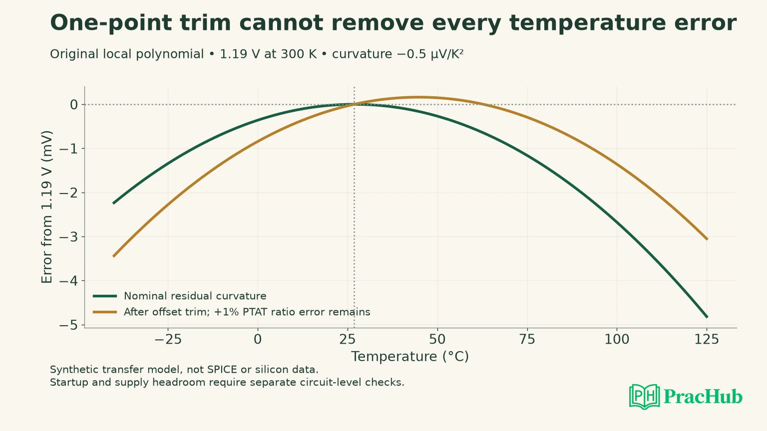
This is a deliberately specific trim model. In a real design, a resistor-ratio trim can change slope as well as nominal output, and a trim code may affect several parameters. State the actuator and its sensitivity rather than saying “trim fixes accuracy.”
Analog Devices' reference application note treats initial accuracy, temperature behavior and other error sources as separate specifications. Use that distinction to ask what an actual production trim measures and controls. A nominal-voltage adjustment cannot be assumed to correct long-term drift, load regulation or every temperature term. AN-82
If asked for two-point trim, explain which two independent errors your model allows you to estimate and which control variables can correct them. Two observations do not create a second physical adjustment knob. Curvature may still require more characterization or another compensation mechanism.
Investigate the unintended zero-current operating point
Temperature cancellation assumes the intended bias currents already exist. Some self-biased reference topologies can also satisfy their equations with no useful current. A DC operating-point solver or an idealized derivation can settle on the desired solution without establishing that power-up reaches it.
Startup circuitry must move the system away from an unintended state and then avoid corrupting normal operation. The exact mechanism depends on the topology. An injected current, a sensing branch or another startup path must have enough authority under relevant supply, process and temperature conditions.
Analog Devices' startup discussion explains that bias and reset dependencies can prevent a reference or regulator from starting as expected. It is a warning to inspect dependency loops, not proof that every bandgap has the same zero-current state or requires the same startup circuit. Startup and bandgap dependencies
An interview answer should distinguish two claims: “the intended equilibrium gives the correct voltage” and “the power-up trajectory reaches that equilibrium.” Our polynomial checks only the first kind of relationship. It contains no current state, supply ramp or startup device and therefore cannot verify the second.
Build a startup matrix with observable exit conditions
Use this original review matrix to turn “test startup” into specific investigations. It is a proposed verification plan, not a report that the tests have been executed. The circuit owner must supply the actual voltage, time and current limits.
| Changed condition | Failure hypothesis | Evidence to request |
|---|---|---|
| Very slow supply ramp | Startup stimulus disappears before bias becomes self-sustaining | Bias and reference waveforms through the ramp |
| Fast ramp with unfavorable initial nodes | Internal nodes remain in an unintended state | Multiple initial conditions and startup-current trace |
| Brownout followed by recovery | Partial discharge prevents a clean restart | Recovery waveform and reset/bias sequence |
| Cold or hot process corner | Startup path becomes too weak or fails to turn off | Corner-specific startup and steady-state current |
| Output load present during startup | Available bias or output current is diverted | Loaded rise, settling and final operating point |
For each case, define when startup has succeeded. Crossing a voltage once is weaker than reaching a valid range and remaining there with the startup path appropriately inactive. Also inspect overshoot and the effect on downstream circuits; a final correct DC value can conceal an unacceptable transient.
Avoid a universal claim that adding more startup current is always safer. A path that remains active can alter reference voltage, increase supply sensitivity or waste power. The desired behavior includes both reaching the operating point and relinquishing control afterward.
Report drift with a declared range and denominator
If asked to convert the temperature curve into a ppm-per-degree figure, first identify the definition being requested. A box-style range metric uses the maximum minus minimum output across the specified interval, divided by a reference voltage and the interval width. A local derivative at 300 K is a different quantity.
Our nominal model has zero local slope at 300 K while still varying by millivolts elsewhere. Reporting only that local zero would conceal the range behavior. Conversely, a range metric does not identify where the worst error occurs or whether the curve is monotonic.
Keep the trim temperature, measurement points and nominal denominator with the reported result. A sparse sweep can miss a maximum between its sampled temperatures. The local polynomial can be inspected analytically; a real reference requires a justified characterization procedure and uncertainty estimate. No production drift specification is inferred from our four-row table.
Connect temperature accuracy to the rest of the circuit
Ask about supply headroom before interpreting the temperature curve. The amplifier, mirrors and transistors must remain in their intended regions. A nominal equation can remain tidy while a low supply prevents the actual circuit from establishing the assumed currents.
Loading belongs in the same review. If the reference drives another block directly, current drawn from the reference node may disturb the relationship that creates the output. A buffer introduces its own offset, noise, stability and startup requirements. It does not remove the need for an error budget.
For trim codes, check range, resolution and monotonicity against the errors being corrected. A code that reaches the nominal target on one sample does not establish adequate range across process. Likewise, a fine code step is not useful if the measurement uncertainty exceeds the adjustment it is meant to resolve.
Name separate evidence for temperature behavior, supply sensitivity, load behavior and startup. It does not compress all four into a single accuracy percentage. Our local calculation gives a transparent starting point for the temperature portion only.
Practice a derivation and a design review
The first two PracHub records below address RF/analog or thermal fundamentals. The other records support explaining ownership, rebuilding decisions and technical trade-offs. They are not a dedicated bandgap question bank or predictions of an employer's questions.
| PracHub question | Rehearsal focus |
|---|---|
| Explain RF/analog IC interview fundamentals | Explain the device assumptions before a reference-temperature derivation. |
| Explain thermal and signal fundamentals | Check absolute temperature, local slope and the limits of the thermal model. |
| Taking Ownership of a Technically Risky Project | Project practice: show who owns a startup risk and its verification. |
| Explain What You Would Change When Rebuilding a Technical Project | Project practice: name what a revised trim or startup design would change. |
| Explain Technical Tradeoffs in a Project You Led | Communication practice: defend a concrete accuracy versus complexity trade-off. |
Use the RF/analog fundamentals question to derive m from the stated slope and density ratio. Then ask a partner to change the trim mechanism or supply ramp. Identify which parts of your answer remain valid and which require circuit-level evidence.
Sources and Further Reading
- Analog Devices University: bandgap reference activity
- Analog Devices AN-82: understanding and applying voltage references
- Analog Devices: self-starting, reset dependencies and bandgaps
Sources checked November 3, 2026. The numerical temperature model and proposed startup matrix are original teaching assets, with separate verification limits.
Comments (0)