Op-Amp Stability Interview: Noise Gain, Loop Gain, and Capacitive Loading
Quick Overview
Explain op-amp stability through noise gain, loop crossover and capacitive loading, then compare two calculated small-signal transient responses. Primary references, original examples and explicit evidence limits support focused preparation.
For an op-amp stability interview, identify the feedback path, calculate noise gain and inspect loop gain at its unity crossing. A capacitive load can add phase lag, while a compensation change can improve the transient response at the cost of bandwidth, noise or load accuracy. Signal gain alone does not settle the question.
The original two-pole example below calculates that trade-off and checks its small-signal step response. PracHub's RF/analog fundamentals question supplies broader discussion practice; the numerical assumptions here make the stability argument independently checkable.
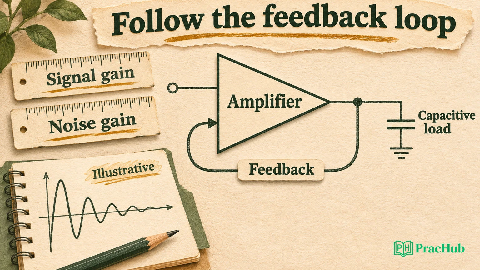
Manufacturer references support the feedback principles. The model parameters, network values and computed responses are synthetic. This is a local linear-system calculation, not a named-device recommendation, SPICE result or bench measurement. No candidate-report set establishes a particular employer's format or question frequency.
Separate the five gains before reading a plot
Open-loop gain A describes the amplifier before closing the external feedback loop. Feedback factor β describes how the output returns to the error input. Loop gain is Aβ. Noise gain is the reciprocal of β under the specified linear feedback network; signal gain describes the desired input-to-output transfer.
For a simple inverting voltage-feedback amplifier with input resistor Rg and feedback resistor Rf, the ideal signal gain is −Rf/Rg. The noise gain is 1 + Rf/Rg. An inverting signal gain of −1 therefore has noise gain two, not minus one and not unity.
Analog Devices' MT-033 explains these distinctions and the use of noise gain when assessing voltage-feedback amplifier stability. Its resistive examples must be generalized to impedances when the feedback network contains capacitors. Do not transfer the same reasoning unchanged to every current-feedback architecture. MT-033
Define where the independent signal source is set to zero when evaluating the feedback network. An omitted source impedance or shunt capacitance can change β. A diagram that labels only an amplifier triangle and “gain = 1” hides the information needed for a stability answer.
Explain how a capacitive load changes the loop
A real amplifier has nonzero output impedance. A load capacitance interacting with that impedance can introduce additional frequency dependence and phase lag. Whether it materially reduces stability margin depends on the amplifier, feedback arrangement, load and existing compensation.
Analog Devices' capacitive-loading article describes this mechanism and several compensation approaches. It does not supply a universal resistor value or guarantee that any ringing waveform has the same cause. Check the device’s loaded response and recommended operating conditions. Capacitive-loading techniques
For the original exercise, represent the loaded amplifier with two real poles. Set DC open-loop gain to 100,000, the first pole to 10 Hz and the second to 100 kHz. Treat the second pole as an illustrative load-related effect. An output resistance of 100 Ω and capacitance about 15.915 nF would produce that simple RC frequency.
The RC mapping is a teaching approximation. Real output impedance varies with frequency, and a load can introduce zeros and other dynamics. We are not claiming that attaching this capacitance to any commercial amplifier produces exactly the model used below.
Calculate crossover and phase margin
Use constant noise gain NG, so β = 1/NG. The model's loop gain is the two-pole open-loop transfer divided by NG. Solve for the frequency at which its magnitude equals one, then calculate the phase there.
A(f) = 100000 / [(1 + j f/10)(1 + j f/100000)]
L(f) = A(f) / NG
Find fc such that |L(fc)| = 1
Phase margin = 180° + phase[L(fc)]
At noise gain two, the calculated unity-loop crossing is about 212.719 kHz, with phase margin about 25.18 degrees. The crossing is already above the second pole, so both poles contribute substantial lag. At noise gain ten, crossover moves down to about 78.615 kHz and phase margin rises to about 51.83 degrees.
| Constant noise gain | Unity-loop crossing | Phase margin | Normalized step overshoot |
|---|---|---|---|
| 2 | 212.719 kHz | 25.18° | 48.63% |
| 10 | 78.615 kHz | 51.83° | 16.30% |
These are results from the original model, not values from a datasheet. They show why moving the crossover can change the transient. They do not establish a universal phase-margin threshold that guarantees acceptable behavior under every load, operating point or nonlinear event.
Keep the frequency units consistent. A transfer function written in s uses angular frequencies in radians per second, whereas the expression above uses frequency ratios in hertz. Mixing a pole in hertz with an s-domain coefficient can shift a numerical result by a factor of 2π.
Change noise gain while preserving ideal signal gain
Increasing a noninverting stage's closed-loop gain would also change its signal gain. That may be unacceptable for a required unity-magnitude signal path. A more revealing interview follow-up asks whether the feedback network can change noise gain without changing that ideal signal gain.
For an inverting stage, choose Rf = Rg = 10 kΩ. With an ideal zero-impedance signal source, the ideal signal gain is −1 and noise gain is two. Add a resistor R3 from the inverting summing node to ground. The ideal signal transfer remains −Rf/Rg because that node is a virtual ground under the ideal approximation.
For noise-gain analysis, the source is zeroed, and Rg is now in parallel with R3. Choosing R3 = 1.25 kΩ gives a parallel resistance about 1.111 kΩ. The resulting noise gain is 1 + 10/1.111 = 10.
The modification also changes noise and error contributions. Finite loop gain changes signal accuracy, and the added resistor contributes thermal noise. Input voltage noise and offset are multiplied by the changed noise gain. The source must also meet the assumed impedance condition; a real source can alter the network.
Our model keeps the ideal signal magnitude one while using the corresponding NG in the closed-loop denominator. That isolates the transient comparison. An implementation still needs a complete noise, offset, loading and bandwidth review before adopting the change.
Check the step response independently of the margin calculation
We used SciPy to solve the unity-loop crossing numerically and to calculate the closed-loop step response from the transfer-function denominator. All closed-loop poles in both modeled cases have negative real parts. Both responses settle in this model, but the lower-margin case rings much more strongly.
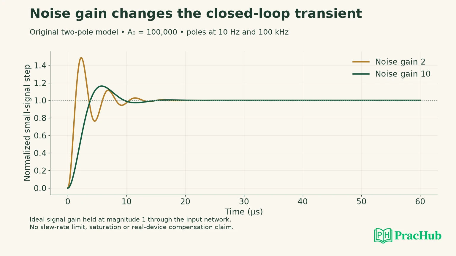
The plotted response is normalized to each case's DC magnitude. That makes transient shape comparable without hiding the fact that finite open-loop gain gives a small static gain error. The calculated DC magnitudes are about 0.999980 and 0.999900 for the modeled unity-magnitude signal path.
The overshoot values are approximately 48.63 percent and 16.30 percent. They describe small-signal linear responses sampled in this calculation. They do not include slew-rate limiting, output-current limits, saturation recovery, common-mode violations or supply behavior.
A similar bench waveform does not establish the same pole locations. Ask whether changing step amplitude changes the response shape. Strong amplitude dependence can point to nonlinear limits, so a phase-margin explanation alone may be incomplete.
Evaluate an isolation resistor without losing the sense point
An output series resistor is another possible way to isolate an amplifier from a capacitive load. Identify where feedback senses the output. A resistor outside the sensed node changes load regulation differently from a resistor enclosed by the feedback loop.
If the feedback senses before the resistor, the amplifier regulates its own output node while load current creates a voltage drop across the resistor. A capacitive load also sees an additional RC response. That can improve one stability concern while reducing delivered bandwidth or changing load accuracy.
If feedback senses after the resistor, the resistor and load participate differently in the return path. Do not reuse the same pole sketch without re-deriving β and the effective open-loop path. Dual-feedback compensation adds further frequency dependence and requires its own analysis.
A useful proposed experiment compares several loads and resistor values while checking settling, gain error and output current. Keep the input amplitude and measurement setup controlled. This article has not performed that circuit experiment and does not recommend a particular resistance for an unspecified amplifier.
State the bandwidth trade-off using the right crossing
The lower unity-loop crossing at noise gain ten is not automatically the signal's minus-three-decibel bandwidth. Closed-loop peaking and the network's signal transfer affect that bandwidth. If a requirement specifies signal bandwidth, calculate or measure the signal transfer directly rather than relabeling the loop crossover.
The normalized step comparison also does not establish settling time to an arbitrary accuracy band. A waveform can cross its final value early and then ring outside the required tolerance. State the error band and require the response to remain within it after the settling point.
For a proposed additional check, calculate frequency response and settling under several parameter variations. A typical phase-margin result is weaker than a verified minimum across the relevant load and device conditions. Our two nominal cases illustrate the mechanism; they do not represent a process or temperature corner sweep.
These distinctions help answer a common challenge: why not keep increasing noise gain? Eventually the bandwidth, noise or offset penalty may violate the application requirements. Compensation is a constrained choice among requirements, not a contest to maximize one margin number independently.
Diagnose ringing before declaring a compensation fix
Begin with the operating point. Check input common-mode range, supply rails, required output swing and load current. A waveform distorted by output clipping or current limiting may not be a small-signal stability problem. Reducing amplitude is one way to test whether the observed behavior changes regime.
Next inspect the measurement setup. A probe, cable or receiving stage can add load capacitance or an unintended feedback path. Record where the signal is measured and whether moving the probe changes the circuit. A convincing diagnosis accounts for the instrument as part of the setup.
Then compare a measured or simulated loop response with the intended model. Identify the unity crossing and phase behavior rather than relying only on a rate-of-closure slogan. If there are multiple crossings or significant delay, the simple two-pole reasoning may not be sufficient.
Finally, evaluate the compensation against the signal requirement. Less overshoot may be useful, but a slower response can miss a settling deadline. The noise-gain change here also increases input-voltage-noise amplification; the manufacturer's noise discussion explains why those contributions need their own budget. Op-amp noise
Practice a defensible stability explanation
The RF/analog and thermal records below support device-level fundamentals. The other records develop project depth, investigation and communication. They are not a dedicated op-amp stability bank or predictions of an employer's questions; the worked model supplies the focused numerical practice.
| PracHub question | Rehearsal focus |
|---|---|
| Explain RF/analog IC interview fundamentals | Relate Bode reasoning to the actual amplifier feedback network. |
| Explain thermal and signal fundamentals | Check signal and noise units while keeping the stability problem distinct. |
| Explain Your Most Technically Complex Project | Project practice: explain the most complex feedback decision in plain terms. |
| Hiring Manager Behavioral Round: Project Impact, Influence, Communication, and Setbacks | Investigation practice: distinguish measurements, hypotheses and setbacks. |
| Present a Technically Challenging Project | Communication practice: connect a compensation choice with its remaining limits. |
Use the RF/analog fundamentals question to explain why an inverting gain of −1 has noise gain two. Then change the load or feedback sense point and say which transfer function must be recalculated. End with the measurement that would distinguish your hypothesis from overload or probe-induced behavior.
Sources and Further Reading
- Analog Devices: capacitive loading and compensation techniques
- Analog Devices MT-033: voltage-feedback gain and bandwidth
- Analog Devices: op-amp noise and circuit contributions
Sources checked November 3, 2026. The numerical loop and transient results are explicitly idealized; real-device stability requires additional evidence.
Comments (0)